Machine Learning in Production
I enrolled and successfully completed the Machine Learning Engineering for Production - Specialisation from Coursera. This blog post aims to give a review of the course and the topics discussed, it’s mostly based on the notes I took during the video lectures. The course covers a wide range of topics and it can feel overwhelming, which is another reason for me to write these review notes.
The specialisation follows the “Steps of a Machine Learning project” which is introduced in the first course and is followed throughout the 4 courses. Some of the concepts are brought up several times during the specialisation and in different courses, they are first briefly introduced and then shown in different contexts and with different levels of detail.
The specialisations tends to focus too much on TensorFlow-related practical demonstrations for the concepts and challenges presented throughout the course, but there are also many references to other software projects for the different challenges presented not relying on Tensorflow.
The specialisation is organised into 4 courses, and I will describe each one separately. I personally enjoyed most the 3rd and 4th courses, it’s where the instructors go into more deep practical details. Some topics are more detailed in my notes than others due to my personal interest or the novelty of the topic for me.
1 - Introduction to Machine Learning in Production
The first course is a high-level introduction to the topics covered in the specialisation, it briefly goes through the different steps of a Machine Learning Project, which are then detailed in the next courses.
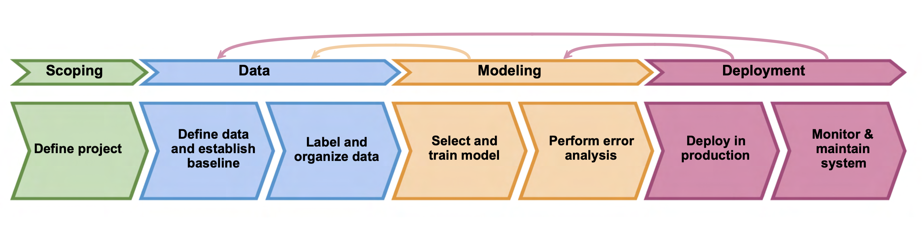
Scoping: the definition of an ML project. Identifying the problem, doing due diligence on the feasibility and value, and considering possible ethical concerns, milestones, and metrics.
Data: introduction to the definition of the data used in the project and an expected baseline, how to label and organize the data: meta-data, data provenance and lineage, balanced train/dev/test splits.
Modelling: how to approach the modelling of the data to solve the problem assuring the algorithm does well on the training data and test data but also positively impacts any business metrics. Auditing the framework by brainstorming ways the system might go wrong, e.g.: performance on subsets of data (e.g., ethnicity, gender), the prevalence of specific errors/outputs, and performance on rare classes.
Deployment: deployment vs. maintenance and deployment patterns:
- Shadow mode: model is deployed and make predictions in the background, and those are only used to evaluate the quality.
- Canary deployment: roll out to a small fraction (say 5%) of traffic initially monitor the system and ramp up traffic gradually.
- Blue-Green deployment: router sends a request to old/blue or to new/green, it enables easy rollback. Monitoring: software/hardware metrics, input metrics, output metrics, thresholds for alarms, adapt metrics and thresholds over time.
2 - Machine Learning Data Lifecycle in Production
This course focuses mostly on the data aspect of a Machine Learning project, and it’s organised into 4 main topics
Collecting, Labelling, Validating (slides)
The main focus of this topic is on the importance of data: the data pipeline, and data monitoring. It starts by explaining the data collection and labelling process, focusing on understanding the data source, the consistency of values, units and data types, and detecting outliers, errors and inconsistent formatting. Mentions privacy and fairness aspects in the data collection, and the use of process feedback using logging tools, such as logstash and fluentd.
Mentions the problems with data, particularly the drift in data, which can be a consequence of trends and seasonality. The impact on the distribution of features and the relative importance of features. Here the instructors explain in great detail the concepts:
Data Drift: changes in data over time, i.e.: changes in the statistical properties of the features over time due to seasonality, trends or unexpected events.
Concept Drift: changes in the statistical properties of the labels over time, i.e.: mapping to labels in training remains static while the real-world changes.
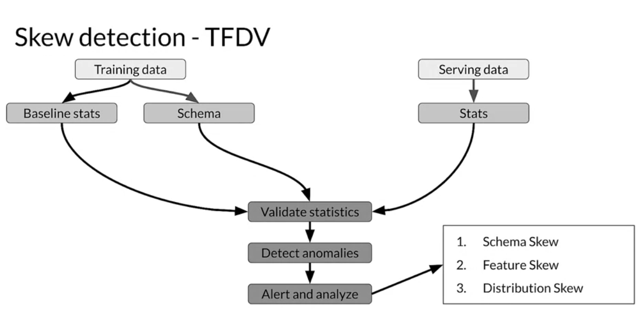
Schema Skew: training and service data do not conform to the same schema, e.g.: getting an integer when expecting a float, empty string vs None
Distribution Skew: divergence between training and serving datasets, dataset shift caused by covariate/concept shift
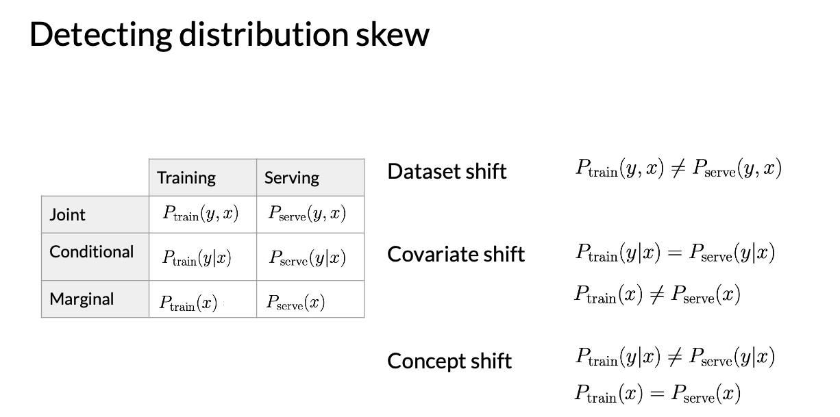
Dataset shift: the joint probability of features \(x\) and labels \(y\) is not the same during training and serving
Covariate shift: a change in the distribution of the input variables present in training and serving data. In other words, it’s where the marginal distribution of features \(x\) is not the same during training and serving, but the conditional distribution remains unchanged.
Concept shift: refers to a change in the relationship between the input and output variables as opposed to the differences in the data distribution or input. It’s when the conditional distribution of labels \(y\) and n features \(x\) are not the same during training and serving, but the marginal distribution features \(x\) remain unchanged.
Software Tools
Feature Engineering (slides)
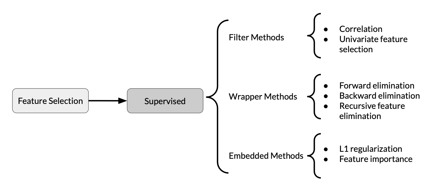
An overview of the pre-processing operations and feature engineering techniques, e.g.: feature scaling, normalisation and standardisation, bucketing/binning. Also, a good summarisation of the techniques to reduce the dimensionality of features: PCA, t-SNE and UMAP. Lastly, how to combine multiple features into a new feature and the feature selection process.
Data Storage (slides)
This chapter deals with the data journey, accounting for data and model evolution and using metadata to track changes in data in the ML pipeline. How a schema to hold data can evolve and how to keep track of those changes, it also introduces the concept of feature stores, as well as Datawarehouse (OLAP) vs. Databases (OLTP) and data lakes.
Advanced Labelling, Augmentation and Data Preprocessing (slides)
The last topic covers data labelling and data augmentation techniques. Semi-Supervised Labelling, and briefly introduce graph-based label propagation, combines supervised and unsupervised data.
For Active Learning, a few strategies to select the best samples to be annotated by a human are introduced and explained:
- Margin sampling: label points the current model is least confident in.
- Cluster-based sampling: sample from well-formed clusters to “cover” the entire space.
- Query-by-committee: train an ensemble of models and sample points that generate disagreement.
- Region-based sampling: Runs several active learning algorithms in different partitions of the space.
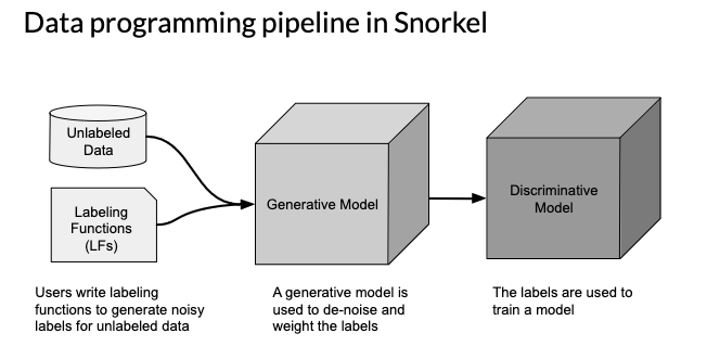
Lastly, for Weak Supervision, the instructors give the example of Snorkel:
- Start with unlabelled data, without ground-truth labels
- One or more weak supervision sources
- A list of heuristics that can automate labelling, typically provided by subject matter experts
- Noisy labels have a certain probability of being correct, but not 100%
- Objective: learn a generative model to determine weights for weak supervision sources
- Learn a supervised model
This topic also briefly explains how to do data augmentation techniques, mostly for images, and about windowing strategies for time series.
3 - Machine Learning Modelling Pipelines in Production
The 3rd course on this specialisation is the longest one covering 5 topics and was also the one that brought, for me, the most interesting topics from all the 4 courses.
Neural Architectural Search and Auto ML (slides)
The first chapter covers automatic parameter tuning. It describes briefly different strategies to find the best hyperparameters (i.e.: set before launching the learning process and not updated in each training step):
- Grid Search
- Random Search
- Bayesian Optimisation
- Evolutionary Algorithms
- Reinforcement Learning
Shows how the hyperparameters can be tuned with Keras Tuner, and it finishes by talking more broadly about the ML topic and the services provided by cloud providers to perform AutoML.
Model Resource Management Techniques (slides)
This one was of particular interest to me, mainly because all of the subjects covered deal with how to make a model more efficient in terms of CPU/GPU needs. Essentially through methods of dimensionality reduction, quantisation and pruning.
Dimensionality Reduction: there’s a brief explanation about the curse of dimensionality and the Hughes effect as motivation for dimensionality reduction, which is can be tackled with manual feature reduction techniques, and the instructors give a few examples and also explain and introduce a few algorithms:
- Unsupervised:
- Principal Components Analysis (PCA)
- Latent Semantic Indexing/Analysis (LSI and LSA) / Singular-Value Decomposition (SVD)
- Independent Component Analysis (ICA)
- Non-Negative Matrix Factorisation (NMF)
- Latent Dirichlet Allocation (LDA)
Quantisation and Pruning
As the instructors explain, one of the motivation reasons for reducing model sizer is the deployment of ML models in IoT and mobile devices.
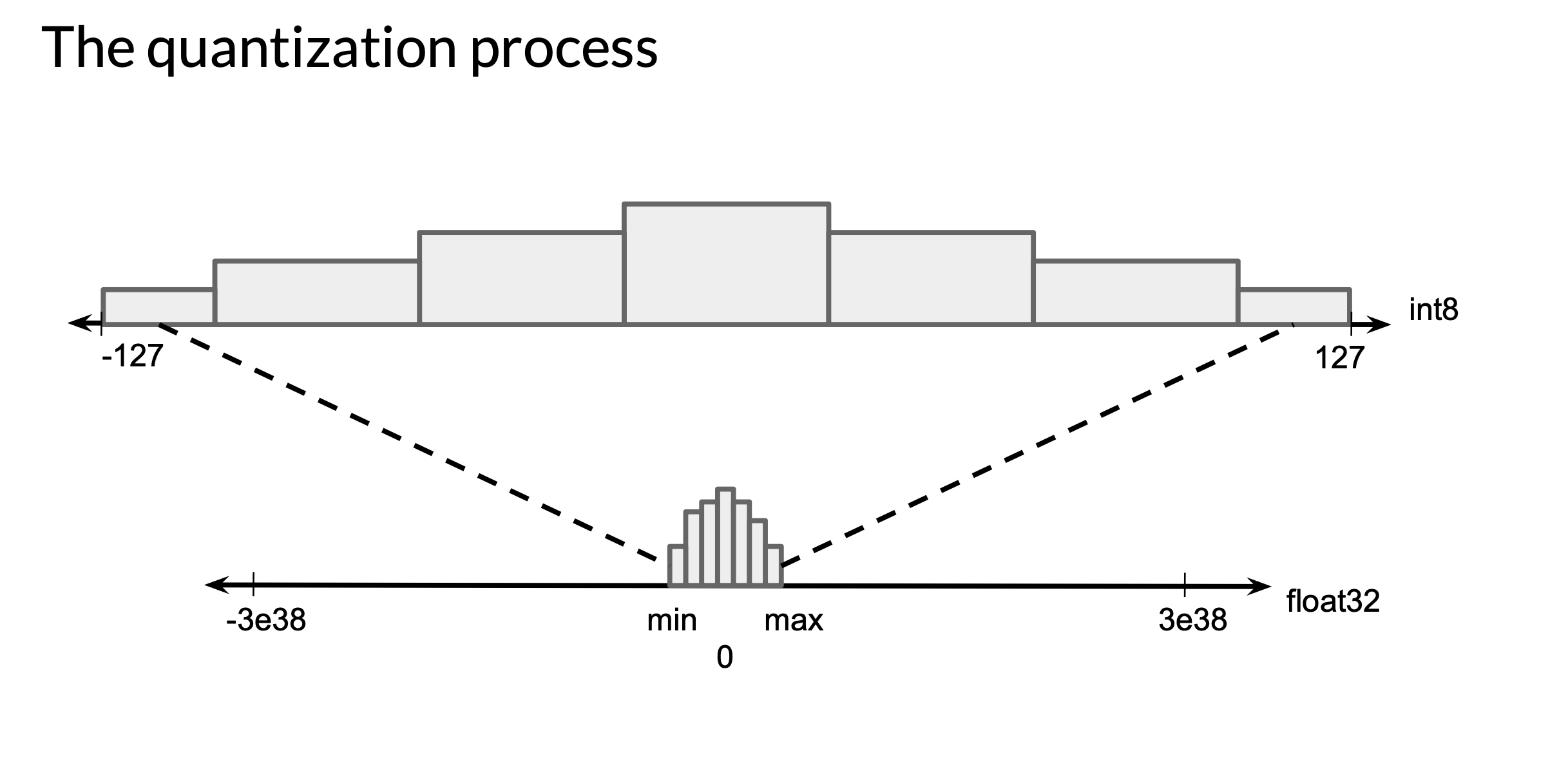
In a nutshell what post-training quantisation does is to efficiently convert or quantise the weights from floating point numbers to integers. This might reduce the precision representation and incur a small loss in model accuracy but significantly reduces the model size making it more feasible to run on a memory-constrained device.
Pruning aims to reduce the number of parameters and operations involved in generating a prediction by removing network connections, this reduces the model capacity, but also its size and complexity.
The instructors also make a mention The Lottery Ticket Hypothesis: Finding Sparse, Trainable Neural Networks with the hypothesis that “a randomly-initialised, dense neural network contains a subnetwork that is initialised such that — when trained in isolation — it can match the test accuracy of the original network after training for at most the same number of iterations”
Reading:
-
Quantisation and Training of Neural Networks for Efficient Integer-Arithmetic-Only Inference
-
The Lottery Ticket Hypothesis: Finding Sparse, Trainable Neural Networks
High-Performance Modelling and Distillation Techniques (slides)
- High-Performance Modelling:
- distributed training, including a couple of different kinds of parallelism.
- Then we’ll turn to high-performance modelling, including high-performance ingestion.
- Distillation Techniques
- Knowledge Distillation
- Teacher and student model
Model Analysis (slides)
This topic covers the question of what’s next after the model is trained and deployed, and its processing data. Is it performing well? Can we improve it? Has the data changed from the training dataset?
One first aspect is how to compute metrics, most of the time, metrics are calculated on the entire dataset, and slicing deals with understanding how the model is performing on each subset of data. This is demonstrated using Tensorflow Model Analysis to perform top-level aggregate metrics versus slicing.
The chapter then covers different model debugging techniques:
Adversarial Attacks
- Random Attacks: expose models to high volumes of random input data
-
Partial dependence plots
– Python Partial Dependence Plot toolbox
– PyCEBbox
-
Measuring your vulnerability to attack
– Cleverhans: benchmark machine learning systems’ vulnerability to adversarial examples
– Foolbox: lets you easily run adversarial attacks against machine-learning models
Residual Analysis
- Measures the difference between the model’s predictions and ground truth
- Randomly distributed errors are good
- Correlated or systematic errors show that a model can be improved
Model Remediation Techniques
- Model editing: manual tweaks to adapt your use case
- Model assertions: implement business rules that override model predictions
Fairness
- Compute performance metrics at all slices of data
- Evaluate your metrics across multiple thresholds
- If the decision margin is small, report in more detail
Continuous Evaluation and Monitoring
- Training data is a snapshot of the world at a point in time and many types of data change over time.
- Concept drift: loss of prediction quality
- Concept Emergence: a new type of data distribution
- Types of dataset shift: covariate shift and prior probability shift
- Statistical process control
- Sequential analysis
- Error distribution monitoring
- Feature distribution monitoring
Model Interpretability (slides)
This chapter introduces the concept and the importance of explainability in AI mentioning other related subjects such as fairness, privacy and security. But ultimately this chapter presents several methods to understand how and why ML models make certain predictions.
It introduces different categories and properties for model interpretation methods, such as post-hoc: models as black boxes, extract relationships between features and model predictions; or model-specific methods (e.g.: interpretation of regression weights in linear models; it finishes with a detailed description of many agnostic models:
- Partial Dependence Plots
- Permutation Feature Importance
- Shapley Values
- SHAP
- Testing Concept Activation Vectors
- Local Interpretable Model-agnostic Explanations (LIME)
Software
4 - Deploying Machine Learning Models in Production
This chapter deals with deploying a trained model, exposing your model to the world outside, and dealing with incoming data requests. It focuses on metrics to optimize such as Latency, Cost, Throughput
Resources and Requirements for Serving Models (slides)
The introduction for this main chapter, with an overview of machine learning workflows: training, predictions; serving patterns: batch inference, real-time inference; metrics: latency, throughput, cost.
How a model complexity can affect different metrics and a quick overview of serving infrastructures, i.e.: using caching and feature lookup. Model deployments in different hardware (data centers, embedded devices, mobile phones).
The chapter ends with a walkthrough demo of TensorFlow Serving.
Model Serving Architecture (slides)
Compares different patterns and infrastructure choices to deploy a model. It starts with the different aspects of deploying a model on-premises or on the cloud and describes different pre-built servers
- TensorFlow Serving
- NVIDIA Triton Inference Server
- Torch Serve
- Kubeflow KFServing
The topic then describes how horizontal scaling can be achieved with containers and orchestration tools, and helps scale the process of serving a model, they give examples with Kubernetes.
It then describes the paradigm of online inference, i.e.: generating machine learning predictions in real-time upon request and which optimisations can be done to decrease latency and increase throughput, giving special focus to data preprocessing.
The chapter ends with the batch inference paradigm within the context of ETLs and distributed processing.
Model Management and Delivery (slides)
This chapter deals with all the model management activities such as tracking model experiments and model versioning, after this, the chapter transitions into the MLops topic. It starts by giving an ML Solution Lifecycle, bridging ML and IT with MLops:
- Continuous Integration (CI): Testing and validating code, components, data, data schemas, and models
- Continuous Delivery (CD): Deploying model prediction service
- Continuous Training (CT): A process that automatically retrains candidate models for testing and serving
- Continuous Monitoring (CM): Catching errors in production systems, and monitoring production inference data and model performance metrics
A proposal on how to manage model versions, MAJOR.MINOR.PIPELINE
- MAJOR: Incompatibility in data or target variable
- MINOR: Model performance is improved
- PIPELINE: The pipeline of model training is changed
and it describes what a model registry can do.
The chapter ends by going into a very detailed and practical description of Continuous Delivery and Progressive Delivery, an improvement over the former.
Model Monitoring (slides)
The last chapter focuses on the last step of a Machine Learning project. It essentially reviews and consolidates concepts already mentioned in the course, but goes into a bit more detail.
Observability and Logging
The chapter introduces the concept of logging as a way of providing observability of the model. Logging should be used to keep track of the model inputs and predictions and detect potential red flags, e.g.: a feature becoming unavailable, or notable shifts in the distributions. Next, introduces the concept of tracing for ML Systems, mentioning some tools.
Model Decay
It follows with a review of the causes of model decay, data drift: statistical properties of input changes; and concept drift: the relationship between features and label changes, the very meaning of what you are trying to predict changes. Model Decay can be mitigated by first detecting drift through logging of request predictions and responses. By observing the statistical properties of logged data and comparing it with the training data one can detect drift.
Libraries for detecting drift:
Lastly, to mitigate the model drift, we need to deal with data:
- Determine the portion of your training set that is still correct
- Keep the good data, discard the bad, and add new data - OR -
- Discard data collected before a certain date and add new data - OR -
- Create an entirely new training dataset from new data
Model:
- Continue training your model, fine-tuning from the last checkpoint using new data - OR -
- Start over, reinitialise your model, and completely retrain it
Responsible AI
This chapter ends by talking about Responsible AI, mainly:
Best practices:
- Human-Centered Design:
- Model potential adverse feedback early in the design process
- Engage with a diverse set of users and use-case scenarios
- Identify Multiple Metrics
- Analyse your raw data carefully: does your data reflect all your users?
Legal Requirements for Secure & Private AI:
- General Data Protection Regulation (GDPR)
- Informational Harms: unintended or unanticipated leakage of information
- Behavioural Harms: manipulating the behaviour of the model itself, impacting the predictions or outcomes of the model
The chapter ends on the Anonymisation & Pseudonymisation topic, showing examples of how to anonymise data under GPDR, and talking about the Right to Be Forgotten, Right to Rectification and other Rights of the Data Subject, all part of the GPDR.
References
-
1 - Introduction to Machine Learning in Production - Lesson Slides
-
2 - Machine Learning Modeling Pipelines in Production - Lesson Slides
-
3 - Deploying Machine Learning Models in Production - Lesson Slides
-
4 - Machine Learning Data Lifecycle in Production - Lesson Slides
-
Figures 1, 2, 3, 4 and 5 are taken from the slides of the course.
coursera mlops production deployment monitoring 