Document Classification
Classifying a document into a pre-defined category is a common problem, for instance, classifying an email as spam or not spam. In this case there is an instance to be classified into one of two possible classes, i.e. binary classification.
However, there are other scenarios, for instance, when one needs to classify a document into one of more than two classes, i.e., multi-class, and even more complex when each document can be assigned to more than one class, i.e. multi-label or multi-output classification.
In this post, I will show an approach to classify a document into a set of pre-defined categories using different supervised classifiers and text representations. I will use the IMDB dataset of movies. Although the dataset contains several pieces of information about a movie, for the scope of this post I will only use the plot of the movie and the genre(s) on which the movie is classified.
Dataset
In order to create the dataset for this experiment you need to download genres.list and plot.list files from a mirror FTP, and then parse files in order to associate the titles, plots, and genres.
I’ve already done this step, and parsed both files in order to generate a single file, available here movies_genres.csv, containing the plot and the genres associated to each movie.
Pre-processing and cleaning
I started by doing some exploratory analysis on the IMDB dataset
%matplotlib inline

import matplotlib
import numpy as np
import matplotlib.pyplot as plt
import pandas as pd

df = pd.read_csv("movies_genres.csv", delimiter='\t')
df.info()
<class 'pandas.core.frame.DataFrame'>
RangeIndex: 117352 entries, 0 to 117351
Data columns (total 30 columns):
title 117352 non-null object
plot 117352 non-null object
Action 117352 non-null int64
Adult 117352 non-null int64
Adventure 117352 non-null int64
Animation 117352 non-null int64
Biography 117352 non-null int64
Comedy 117352 non-null int64
Crime 117352 non-null int64
Documentary 117352 non-null int64
Drama 117352 non-null int64
Family 117352 non-null int64
Fantasy 117352 non-null int64
Game-Show 117352 non-null int64
History 117352 non-null int64
Horror 117352 non-null int64
Lifestyle 117352 non-null int64
Music 117352 non-null int64
Musical 117352 non-null int64
Mystery 117352 non-null int64
News 117352 non-null int64
Reality-TV 117352 non-null int64
Romance 117352 non-null int64
Sci-Fi 117352 non-null int64
Short 117352 non-null int64
Sport 117352 non-null int64
Talk-Show 117352 non-null int64
Thriller 117352 non-null int64
War 117352 non-null int64
Western 117352 non-null int64
dtypes: int64(28), object(2)
memory usage: 26.9+ MB
We have a total of 117 352 movies and each of them is associated with 28 possible genres. The genres columns simply contain a 1 or 0 depending on whether the movie is classified into that particular genre or not. This means the multi-label binary mask is already provided in this file.
Next, we are going to calculate the absolute number of movies per genre. Note: each movie can be associated with more than one genre, we just want to know which genres have more movies.
df_genres = df.drop(['plot', 'title'], axis=1)
counts = []
categories = list(df_genres.columns.values)
for i in categories:
    counts.append((i, df_genres[i].sum()))
df_stats = pd.DataFrame(counts, columns=['genre', '#movies'])
df_stats| genre | #movies | |
|---|---|---|
| 0 | Action | 12381 |
| 1 | Adult | 61 |
| 2 | Adventure | 10245 |
| 3 | Animation | 11375 |
| 4 | Biography | 1385 |
| 5 | Comedy | 33875 |
| 6 | Crime | 15133 |
| 7 | Documentary | 12020 |
| 8 | Drama | 46017 |
| 9 | Family | 15442 |
| 10 | Fantasy | 7103 |
| 11 | Game-Show | 2048 |
| 12 | History | 2662 |
| 13 | Horror | 2571 |
| 14 | Lifestyle | 0 |
| 15 | Music | 2841 |
| 16 | Musical | 596 |
| 17 | Mystery | 12030 |
| 18 | News | 3946 |
| 19 | Reality-TV | 12338 |
| 20 | Romance | 19242 |
| 21 | Sci-Fi | 8658 |
| 22 | Short | 578 |
| 23 | Sport | 1947 |
| 24 | Talk-Show | 5254 |
| 25 | Thriller | 8856 |
| 26 | War | 1407 |
| 27 | Western | 2761 |
df_stats.plot(x='genre', y='#movies', kind='bar', legend=False, grid=True, figsize=(15, 8))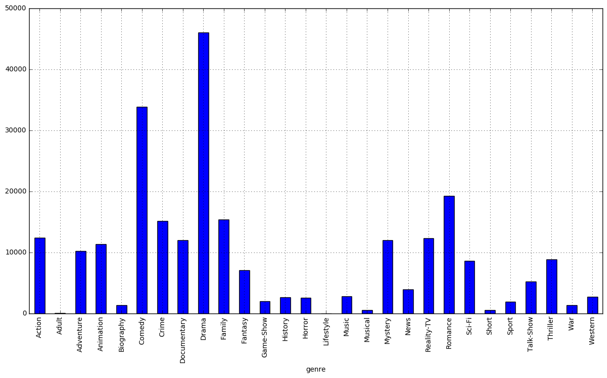
Since the Lifestyle has 0 instances we can just remove it from the data set
df.drop('Lifestyle', axis=1, inplace=True)One thing that notice when working with this dataset is that there are plots written in different languages. Let’s use langedetect tool to identify the language in which the plots are written
from langdetect import detect
df['plot_lang'] = df.apply(lambda row: detect(row['plot'].decode("utf8")), axis=1)
df['plot_lang'].value_counts()
en 117196
nl 120
de 14
da 6
it 6
pt 2
fr 2
no 2
hu 1
es 1
sl 1
sv 1
Name: plot_lang, dtype: int64
There are other languages besides English, let’s just keep English plots, and save this to a new file.
df = df[df.plot_lang.isin(['en'])]
df.to_csv("movies_genres_en.csv", sep='\t', encoding='utf-8', index=False)
Vector Representation and Classification
For vector representation and I will use two Python packages:
To train supervised classifiers, we first need to transform the plot into a vector of numbers. I will explore 3 different vector representations:
- TF-IDF weighted vectors
- word2vec embeddings
- doc2vec embeddings
After having these vector representations of the text we can train supervised classifiers to train unseen plots and predict the genres on which they fall.
TF-IDF
Based on the bag-of-words model, i.e., no word order is kept. I considered TF-IDF weighted vectors, composed of different n-grams size, namely: uni-grams, bi-grams and tri-grams. I also experimentally eliminated words that appear in more than a given number of documents. All these features can be easily configured with TfidfVectorizer class.
The max_df parameter is used for removing terms that appear too frequently, i.e., max_df = 0.50 means “ignore terms that appear in more than 50% of the documents”. The ngram_range parameter selects how large is the sequence of words to be considered.
tfidf__max_df: (0,25 0.50, 0.75)
tfidf__ngram_range: ((1, 1), (1, 2), (1, 3))
Word2Vec
Under this scenario, a movie plot is represented by a single real-value dense vector based on the word embeddings associated with each word. This is done by selecting words from the plot, based on their part-of-speech (PoS)-tags, and then summing their word embeddings and averaging them into a single vector. I used the GoogleNews-vectors, which have a dimension of 300 and are derived from English corpora. For this experiment I selected only adjectives and nouns;
Doc2Vec
Doc2Vec is an extension made over Word2Vec, which tries to model a single document or paragraph as a unique single real-value dense vector. You can read more about it in the original paper. I will use the gensim implementation to derive vectors based on a single document.
At the end of this post, you have a link to the complete code, showing how to generate embeddings with word2vec and doc2vec.
Load pre-processed data:
First, we are going to load the pre-processed and cleaned data into the proper data structures which serve as input for the sklearn classifiers:
data_df = pd.read_csv("movies_genres_en.csv", delimiter='\t')

# split the data, leave 1/3 out for testing
data_x = data_df[['plot']].as_matrix()
data_y = data_df.drop(['title', 'plot', 'plot_lang'], axis=1).as_matrix()
stratified_split = StratifiedShuffleSplit(n_splits=2, test_size=0.33)
for train_index, test_index in stratified_split.split(data_x, data_y):
    x_train, x_test = data_x[train_index], data_x[test_index]
    y_train, y_test = data_y[train_index], data_y[test_index]

# transform matrix of plots into lists to pass to a TfidfVectorizer
train_x = [x[0].strip() for x in x_train.tolist()]
test_x = [x[0].strip() for x in x_test.tolist()]
After loading the data I also split the data into two sets:
- 2/3 ~ 66.6% of the data for tuning the parameters of the classifiers
- 1/3 ~ 33.3% will be used to test the performance of the classifiers
To achieve this I used the StratifiedShuffleSplit class which returns stratified randomised folds, preserving the percentage of samples for each class.
In order to experiment with different features for the text representation and tune the different parameters of the classifiers I used sklearn Pipeline and GridSearchCV. I also use another class, to help transform binary classifiers into multi-label/multi-output classifiers, concretely OneVsRestClassifier, this class wraps ups the process of training a classifier for each possible class.
I considered the following supervise algorithms
- Naive Bayes
- SVM linear
- Logistic Regression
Note that Naive Bayes and Logistic Regression inherently support multi-class, but we are in a multi-label scenario, that’s the reason why even these are wrapped in the OneVsRestClassifier process.
Naive Bayes
pipeline = Pipeline([
    ('tfidf', TfidfVectorizer(stop_words=stop_words)),
    ('clf', OneVsRestClassifier(MultinomialNB(
        fit_prior=True, class_prior=None))),
])
parameters = {
    'tfidf__max_df': (0.25, 0.5, 0.75),
    'tfidf__ngram_range': [(1, 1), (1, 2), (1, 3)],
    'clf__estimator__alpha': (1e-2, 1e-3)
}
SVM linear
pipeline = Pipeline([
    ('tfidf', TfidfVectorizer(stop_words=stop_words)),
    ('clf', OneVsRestClassifier(LinearSVC()),
])
parameters = {
    'tfidf__max_df': (0.25, 0.5, 0.75),
    'tfidf__ngram_range': [(1, 1), (1, 2), (1, 3)],
    "clf__estimator__C": [0.01, 0.1, 1],
    "clf__estimator__class_weight": ['balanced', None],
}
Logistic Regression
pipeline = Pipeline([
    ('tfidf', TfidfVectorizer(stop_words=stop_words)),
    ('clf', OneVsRestClassifier(LogisticRegression(solver='sag')),
])
parameters = {
    'tfidf__max_df': (0.25, 0.5, 0.75),
    'tfidf__ngram_range': [(1, 1), (1, 2), (1, 3)],
    "clf__estimator__C": [0.01, 0.1, 1],
    "clf__estimator__class_weight": ['balanced', None],
}
Parameter tunning through GridSearchCV
We then pass the built pipeline into a GridSearchCV object, and find the best parameters for both the bag-of-words representation and the classifier.
grid_search_tune = GridSearchCV(
    pipeline, parameters, cv=2, n_jobs=2, verbose=3)
grid_search_tune.fit(train_x, train_y)

print
print("Best parameters set:")
print grid_search_tune.best_estimator_.steps
print

# measuring performance on test set
print "Applying best classifier on test data:"
best_clf = grid_search_tune.best_estimator_
predictions = best_clf.predict(test_x)

print classification_report(test_y, predictions, target_names=genres)
Results
TF-IDF
Naive Bayes best parameters set:
    TfidfVectorizer: max_df=0.25, ngram_range=(1, 3)
    MultinomialNB: alpha=0.001

Linear SVM best parameters set:
    TfidfVectorizer: max_df=0.25 ngram_range=(1, 2)
    LinearSVC:  C=1, class_weight='balanced'

LogisticRegression best parameters set:
    TfidfVectorizer:  max_df=0.75, ngram_range=(1, 2)
    LogisticRegression: C=1, class_weight='balanced'


                     precision    recall   f1-score

Naive Bayes            0.95        0.76      0.84
Linear SVM             0.89        0.86      0.87
LogisticRegression     0.70        0.89      0.78
Word2Vec
Linear SVM best parameters set:
    LinearSVC:  C=1, class_weight=None

LogisticRegression best parameters set:
    LogisticRegression: C=1, class_weight=None

                     precision    recall   f1-score

Linear SVM             0.68        0.37      0.45
LogisticRegression     0.67        0.40      0.48
Doc2Vec
Linear SVM best parameters set:
    LinearSVC:  C=0.1, class_weight=None

LogisticRegression best parameters set:
    LogisticRegression: C=1, class_weight=None

                     precision    recall   f1-score

Linear SVM             0.69        0.31      0.40
LogisticRegression     0.65        0.36      0.45
Conclusion
The best results are achieved with a Linear SVM and TF-IDF representation of the text, below you can see the results by genre.
Best parameters set:
    TfidfVectorizer(max_df=0.25, ngram_range=(1, 2))
        LinearSVC(C=1, class_weight='balanced')

              precision    recall  f1-score   support

     Action       0.89      0.84      0.86      4046
      Adult       1.00      0.67      0.80        21
  Adventure       0.89      0.81      0.85      3415
  Animation       0.92      0.86      0.89      3780
  Biography       0.95      0.58      0.72       491
     Comedy       0.89      0.87      0.88     11236
      Crime       0.86      0.90      0.88      4974
Documentary       0.84      0.83      0.84      3986
      Drama       0.89      0.94      0.91     15110
     Family       0.89      0.84      0.86      5160
    Fantasy       0.90      0.79      0.84      2381
  Game-Show       0.95      0.87      0.91       730
    History       0.86      0.70      0.77       853
     Horror       0.93      0.66      0.77       826
      Music       0.92      0.82      0.87       951
    Musical       0.96      0.58      0.73       190
    Mystery       0.82      0.85      0.84      3918
       News       0.91      0.83      0.87      1337
 Reality-TV       0.89      0.85      0.87      4057
    Romance       0.90      0.90      0.90      6472
     Sci-Fi       0.90      0.83      0.86      2853
      Short       1.00      0.48      0.65       183
      Sport       0.91      0.73      0.81       616
  Talk-Show       0.89      0.87      0.88      1775
   Thriller       0.86      0.78      0.82      2914
        War       0.91      0.79      0.84       447
    Western       0.96      0.86      0.91       874

avg / total       0.89      0.86      0.87     83596
The embedding method shows very low results, the representation based on the word2vec was just a naive way to get sentence embeddings, more robust methods could be explored like concatenating each word’s vector into a single vector and giving it as input to a neural network.
The doc2vec vectors were generated with gensim out-of-the-box, some parameter tuning on the vectors generation process might give better results.
Also, word2vec and doc2vec, since they have a much lower dimension, i.e. 300 compared to 50 000 up to 100 000 of the TF-IDF weighted vectors, could probably be achieved with a non-linear kernel.
The full code for this post is available on my GitHub:
https://github.com/davidsbatista/text-classification
Related posts
multi-label-classification scikit-learn tf-idf word2vec doc2vec 