The Attention Mechanism in Natural Language Processing
The Attention mechanism is now an established technique in many NLP tasks. I’ve heard about it often but wanted to go a bit more deeply and understand the details. In this first blog post - since I plan to publish a few more blog posts regarding the attention subject - I make an introduction by focusing on the first proposal of attention mechanism, as applied to the task of neural machine translation.
Introduction
To the best of my knowledge the attention mechanism within the context of NLP was first presented in “Neural Machine Translation by Jointly Learning to Align and Translate” at ICLR 2015 (Bahdanau et al. 2015).
This was proposed in the context of machine translation, where given a sentence in one language, the model has to produce a translation for that sentence in another language.
In the paper, the authors propose to tackle the problem of a fixed-length context vector in the original seq2seq model for machine translation (Cho et al., 2014)
The classical Sequence-to-Sequence model
The model is composed of two main components: an encoder, and a decoder.
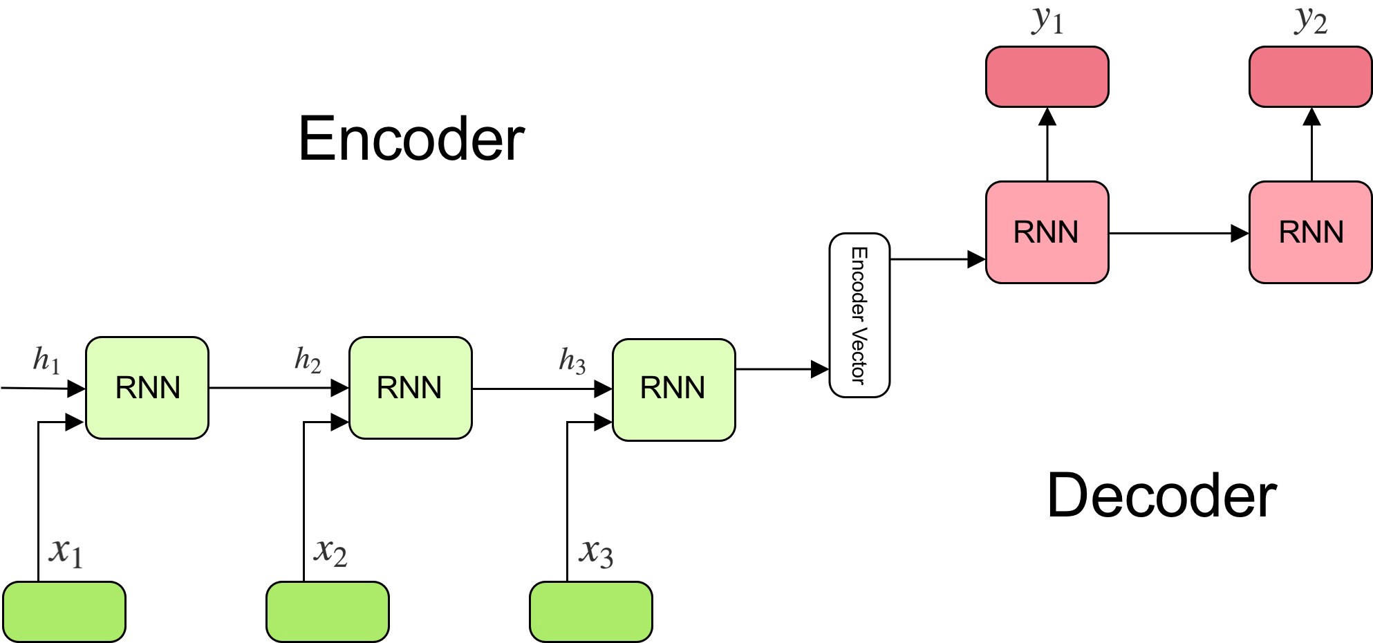
The encoder reads the input sentence, a sequence of vectors \(x = (x_{1}, \dots , x_{T})\), into a fixed-length vector \(c\). The encoder is a recurrent neural network, typical approaches are GRU or LSTMs such that:
\[h_{t} = f\ (x_{t}, h_{t−1})\] \[c = q\ (h_{1}, \dotsc, h_{T})\]where \(h_{t}\) is a hidden state at time \(t\), and \(c\) is a vector generated from the sequence of the hidden states, and \(f\) and \(q\) are some nonlinear functions.
At every time-step \(t\) the encoder produces a hidden state \(h_{t}\), and the generated context vector is modelled according to all hidden states.
The decoder is trained to predict the next word \(y_{t}\) given the context vector \(c\) and all the previously predict words \(\\{y_{1}, \dots , y_{t-1}\\}\), it defines a probability over the translation \({\bf y}\) by decomposing the joint probability:
\[p({\bf y}) = \prod\limits_{i=1}^{x} p(y_{t} | {y_{1}, \dots , y_{t-1}}, c)\]where \(\bf y = \\{y_{1}, \dots , y_{t}\\}\). In other words, the probability of a translation sequence is calculated by computing the conditional probability of each word given the previous words. With an LSTM/GRU each conditional probability is computed as:
\[p(y_{t} | {y_{1}, \dots , y_{t-1}}, c) = g(y_{t−1}, s_{t}, c)\]where, \(g\) is a nonlinear function that outputs the probability of \(y_{t}\), \(s_{t}\) is the value of the hidden state of the current position, and \(c\) the context vector.
In a simple seq2seq model, the last output of the LSTM/GRU is the context vector, encoding context from the entire sequence. This context vector is then used as the initial hidden state of the decoder.
At every step of decoding, the decoder is given an input token and (the previous)
hidden state. The initial input token is the start-of-string
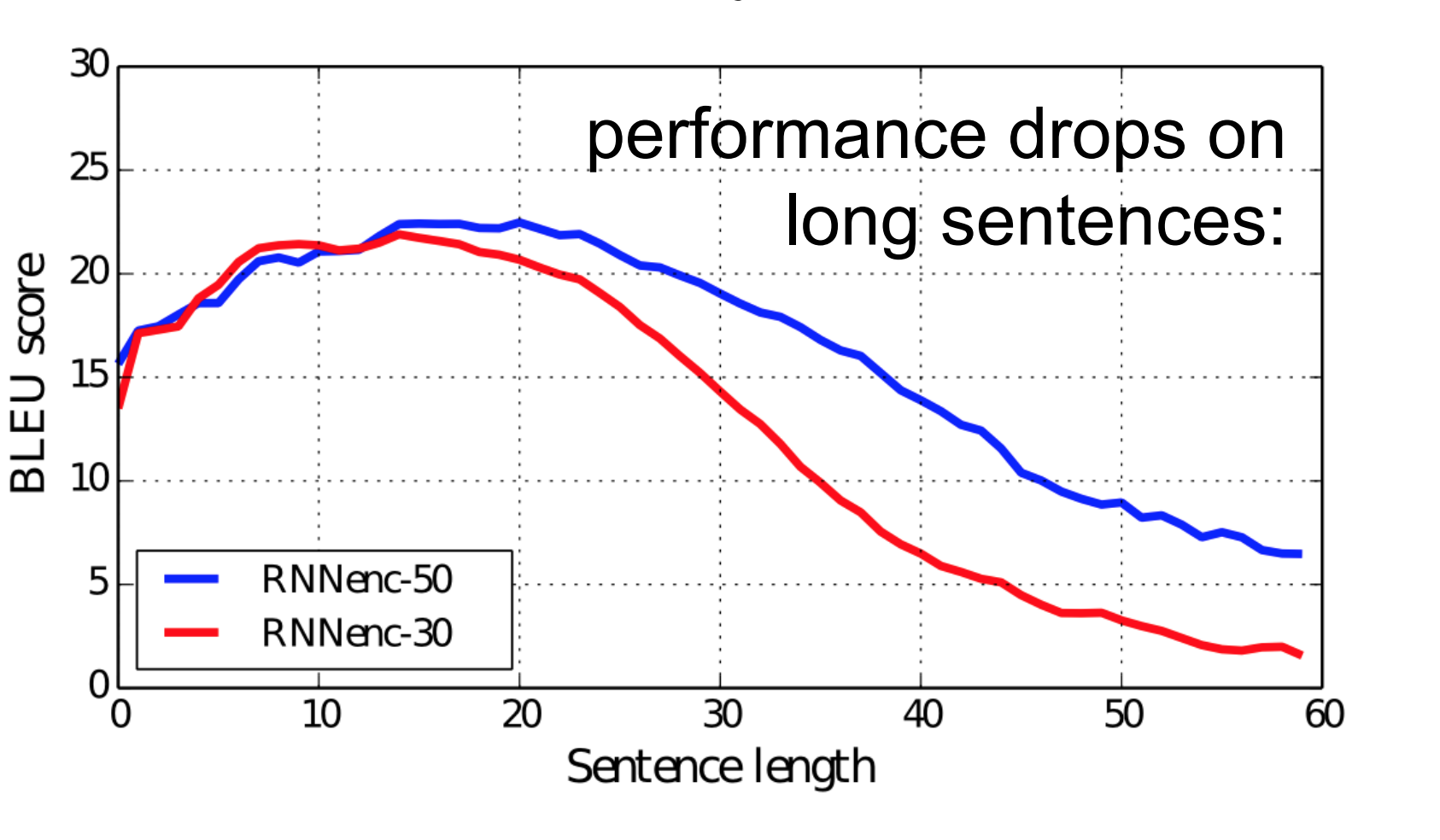
So, the fixed size context-vector needs to contain a good summary of the meaning of the whole source sentence, being this one big bottleneck, especially for long sentences.
Sequence-to-Sequence model with Attention
The fixed-size context-vector bottleneck was one of the main motivations by Bahdanau et al. 2015, which proposed a similar architecture but with a crucial improvement:
“The new architecture consists of a bidirectional RNN as an encoder and a decoder that emulates searching through a source sentence during decoding a translation”
The encoder is now a bidirectional recurrent network with forward and backwards hidden states. A simple concatenation of the two hidden states represents the encoder state at any given position in the sentence. The motivation is to include both the preceding and following words in the representation/annotation of an input word.
The other key element, and the most important one, is that the decoder is now equipped with some sort of search, allowing it to look at the whole source sentence when it needs to produce an output word, the attention mechanism.
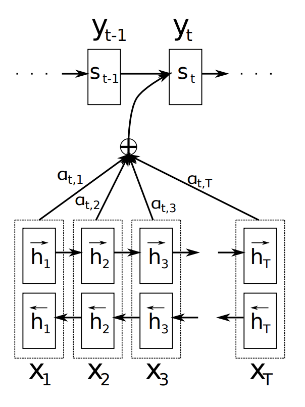
Figure 2 above gives a good overview of this new mechanism. To produce the output word at time \(y_{t}\) the decoder uses the last hidden state from the decoder - one can think about this as some sort of representation of the already produced words - and a dynamically computed context vector based on the input sequence.
The authors proposed to replace the fixed-length context vector by another context vector \(c_{i}\) which is a sum of the hidden states of the input sequence, weighted by alignment scores.
Note that now the probability of each output word is conditioned on a distinct context vector \(c_{i}\) for each target word \(y\).
The new decoder is then defined as:
\[p(y_{t} | {y_{1}, \dots , y_{t-1}}, c) = g(y_{t−1}, s_{i}, c)\]where \(s_{i}\) is the hidden state for time \(i\), computed by:
\[s_{i} = f(s_{i−1}, y_{i−1}, c_{i})\]that is, a new hidden state for \(i\) depends on the previous hidden state, the representation of the word generated by the previous state and the context vector for position \(i\). The remaining question now is, how to compute the context vector \(c_{i}\)?
Context Vector
The context vector \(c_{i}\) is a sum of the hidden states of the input sequence, weighted by alignment scores. Each word in the input sequence is represented by a concatenation of the two (i.e., forward and backward) RNNs hidden states, let’s call them annotations.
Each annotation contains information about the whole input sequence with a strong focus on the parts surrounding the \(i_{th}\) word in the input sequence.
The context vector \(c_{i}\) is computed as a weighted sum of these annotations:
\[c_{i} = \sum_{j=1}^{T_{x}} \alpha_{ij}h_{j}\]The weight \(\alpha_{ij}\) of each annotation \(h_{j}\) is computed by:
\[\alpha_{ij} = \text{softmax}(e_{ij})\]where:
\[e_{ij} = a(s_{i-1,h_{j}})\]\(a\) is an alignment model which scores how well the inputs around position \(j\) and the output at position \(i\) match. The score is based on the RNN hidden state \(s_{i−1}\) (just before emitting \(y_{i}\)) and the \(j_{th}\) annotation \(h_{j}\) of the input sentence
\[a(s_{i-1},h_{j}) = \mathbf{v}_a^\top \tanh(\mathbf{W}_{a}\ s_{i-1} + \mathbf{U}_{a}\ {h}_j)\]where both \(\mathbf{v}_a\) and \(\mathbf{W}_a\) are weight matrices to be learned in the alignment model.
The alignment model in the paper is described as a feed-forward neural network whose weight matrices \(\mathbf{v}_a\) and \(\mathbf{W}_a\) are learned jointly together with the whole graph/network.
The authors note:
“The probability \(\alpha_{ij}h_{j}\) reflects the importance of the annotation \(h_{j}\) with respect to the previous hidden state \(s_{i−1}\) in deciding the next state \(s_{i}\) and generating \(y_{i}\). Intuitively, this implements a mechanism of attention in the decoder.
Resume
It’s now useful to review again visually the attention mechanism and compare it against the fixed-length context vector. The pictures below were made by Nelson Zhao and hopefully will help understand clearly the difference between the two encoder-decoder approaches.
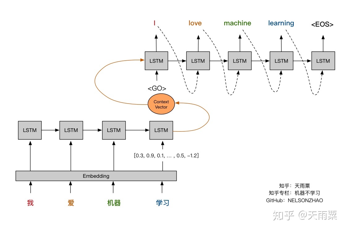
(https://zhuanlan.zhihu.com/p/37290775)
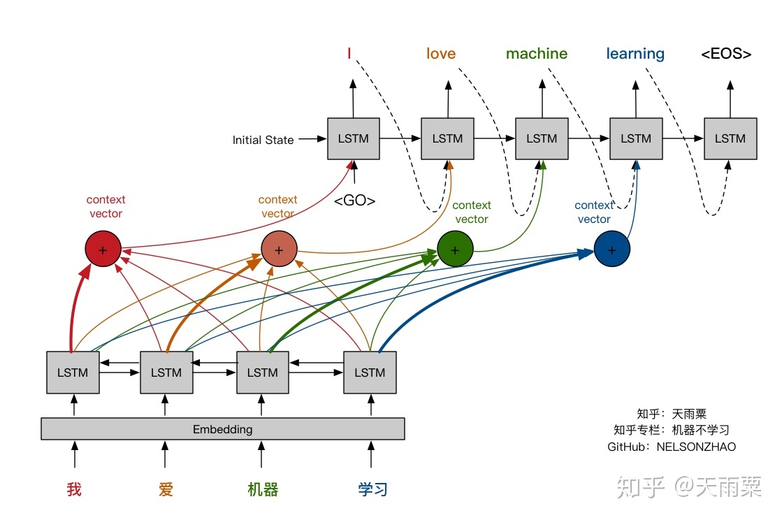
(https://zhuanlan.zhihu.com/p/37290775)
Extensions to the classical attention mechanism
Luong et al. proposed and compared other mechanisms of attention, more specifically, alternative functions to compute the alignment score:
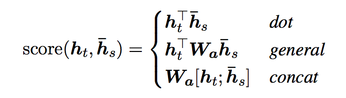
NOTE: the concat is the same as in Bahdanau et al. 2015. But, most importantly, instead of a weighted average over all the source hidden states, they proposed a mechanism of local attention which focus only on a small subset of the source positions per target word instead of attending to all words on the source for each target word.
Summary
This was a short introduction to the first “classical” attention mechanism, in the meantime others were published, such as self-attention or key-value-attention, which I plan to write about in the future.
The attention mechanism was then applied to other natural language processing tasks based on neural networks such as RNN/CNN, such as document-level classification or sequence labelling, which I plan to write a bit more about in forthcoming blog posts.
References
-
[1] An Introductory Survey on Attention Mechanisms in NLP Problems (arXiv.org version)
-
[2] Neural Machine Translation by Jointly Learning to Align and Translate (slides)
-
[3] Effective Approaches to Attention-based Neural Machine Translation (slides)
-
Figure 1 taken from towardsdatascience
-
Figure 2 and 3 taken from Bahdanau et al. 2015
-
Figure 4 and 5 taken from Nelson Zhao blog’s post
-
Figure 6 taken from Luong et al.
attention neural-networks LSTM GRU RNN 