Language Models and Contextualised Word Embeddings
Since the work of Mikolov et al., 2013 was published and the software package word2vec was made public available a new era in NLP started on which word embeddings, also referred to as word vectors, play a crucial role. Word embeddings can capture many different properties of a word and become the de-facto standard to replace feature engineering in NLP tasks.
Since that milestone, many new embedding methods were proposed some of which go down to the character level, and others that take into consideration even language models. I will try in this blog post to review some of these methods, but focusing on the most recent word embeddings which are based on language models and take into consideration the context of a word.
Introduction
This blog post consists of two parts, the first one, which is mainly pointers, simply refers to the classic word embedding techniques, which can also be seen as static word embeddings since the same word will always have the same representation regardless of the context where it occurs. I quickly introduce three embeddings techniques:
- Skip-Gram (aka Word2Vec)
- Glove
- fastText
The second part introduces three news word embedding techniques that take into consideration the context of the word and can be seen as dynamic word embedding techniques, most of which make use of some language model to construct the representation of a word. I try to describe three contextual embeddings techniques:
- ELMO
- FlairEmbeddings
- BERT
Classic Word Embeddings
Efficient Estimation of Word Representations in Vector Space (2013)
Introduced by Mikolov et al., 2013 it was the first popular embedding method for NLP tasks. The paper itself is hard to understand, and many details are left over, but essentially the model is a neural network with a single hidden layer, and the embeddings are actually the weights of the hidden layer in the neural network.
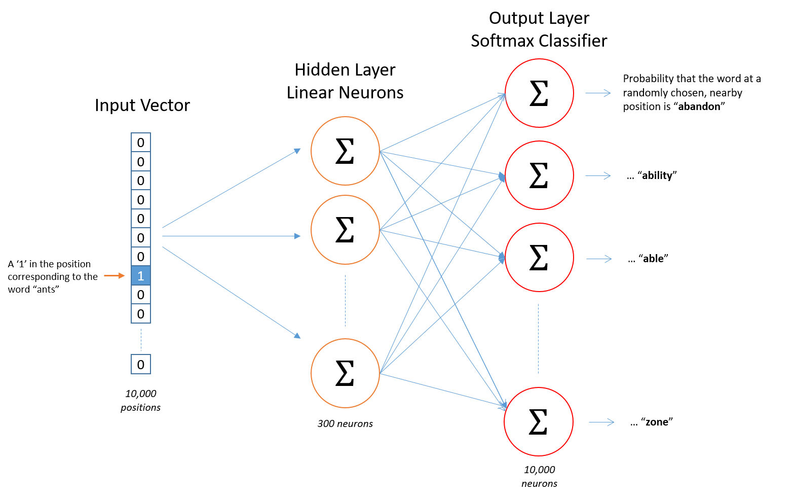
Image taken from http://mccormickml.com/2016/04/19/word2vec-tutorial-the-skip-gram-model/
An important aspect is how to train this network in an efficient way and then is when negative sampling comes into play.
I will not go into detail regarding this one, as the number of tutorials, implementations and resources regarding this technique is abundant on the net, and I will just rather leave some pointers.
Links
- McCormick, C. (2016, April 19). Word2Vec Tutorial - The Skip-Gram Model.
- McCormick, C. (2017, January 11). Word2Vec Tutorial Part 2 - Negative Sampling.
- word2vec Parameter Learning Explained, Xin Rong
- https://code.google.com/archive/p/word2vec/
- Stanford NLP with Deep Learning: Lecture 2 - Word Vector Representations: word2vec
GloVe: Global Vectors for Word Representation (2014)
I will also give a brief overview of this work since there are also abundant resources online. It was published shortly after the skip-gram technique and essentially it starts to make an observation that shallow window-based methods suffer from the disadvantage that they do not operate directly on the co-occurrence statistics of the corpus. Window-based models, like skip-gram, scan context windows across the entire corpus and fail to take advantage of the vast amount of repetition in the data.
Count models, like GloVe, learn the vectors by essentially doing some sort of dimensionality reduction on the co-occurrence counts matrix. They start by constructing a matrix with counts of word co-occurrence information, each row tells how often does a word occur with every other word in some defined context size in a large corpus. This matrix is then factorised, resulting in a lower-dimension matrix, where each row is some vector representation for each word.
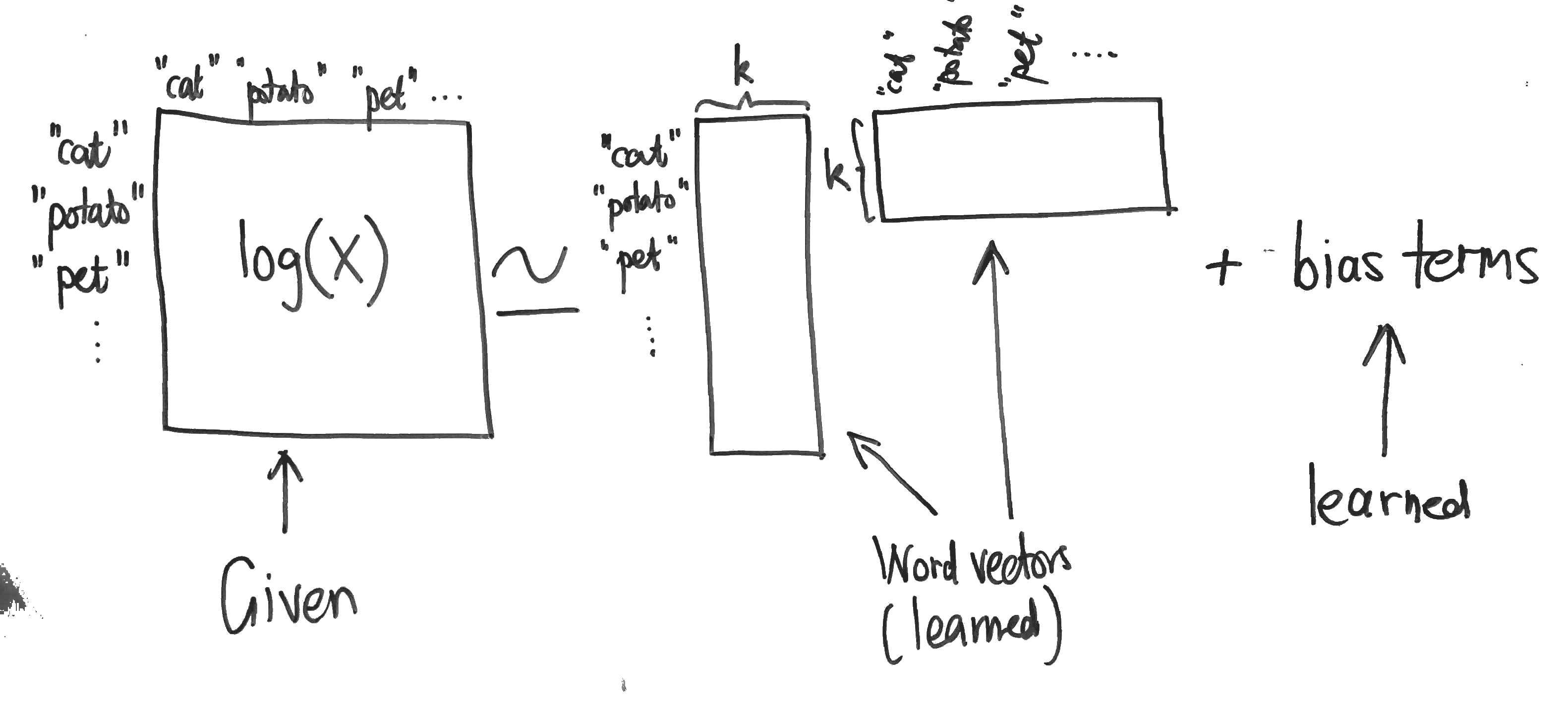
Image taken from http://building-babylon.net/2015/07/29/glove-global-vectors-for-word-representations/
The dimensionality reduction is typically done by minimising some kind of ‘reconstruction loss’ that finds lower-dimension representations of the original matrix and which can explain most of the variance in the original high-dimensional matrix.
Links
- GloVe project at Stanford
- Building Babylon: Global Vectors for Word Representations
- Good summarization on text2vec.org
- Stanford NLP with Deep Learning: Lecture 3 GloVe - Global Vectors for Word Representation
- Paper Dissected: ‘Glove: Global Vectors for Word Representation’ Explained
Enriching Word Vectors with Subword Information (2017)
One drawback of the two approaches presented before is the fact that they don’t handle out-of-vocabulary.
The work of Bojanowski et al, 2017 introduced the concept of subword-level embeddings, based on the skip-gram model, but where each word is represented as a bag of character \(n\)-grams.
Image taken from https://fasttext.cc/
A vector representation is associated with each character \(n\)-gram, and words are represented as the sum of these representations. This allows the model to compute word representations for words that did not appear in the training data.
Each word $w$ is represented as a bag of character $n$-gram, plus special boundary symbols < and > at the beginning and end of words, plus the word $w$ itself in the set of its $n$-grams.
Taking the word where and $n = 3$ as an example, it will be represented by the character $n$-grams:
Links
- https://github.com/facebookresearch/fastText
- Library for efficient text classification and representation learning
Static Word Embeddings fail to capture polysemy
The models presented before have a fundamental problem, which is, they generate the same embedding for the same word in different contexts, for example, given the word bank although it will have the same representation it can have different meanings:
- “I deposited 100 EUR in the bank.”
- “She was enjoying the sunset o the left bank of the river.”
In the methods presented before, the word representation for bank would always be the same regardless if it appears in the context of geography or economics. In the next part of the post, we will see how new embedding techniques capture polysemy.
Contextualised Word-Embeddings
Contextualised word embeddings aim at capturing word semantics in different contexts to address the issue of polysemous and the context-dependent nature of words.
Language Models
Language models compute the probability distribution of the next word in a sequence given the sequence of previous words. LSTMs become a popular neural network architecture to learn these probabilities. The figure below shows how an LSTM can be trained to learn a language model.
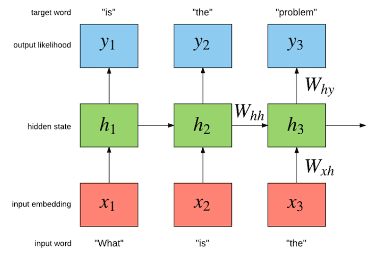
Image taken from http://torch.ch/blog/2016/07/25/nce.html
A sequence of words is fed into an LSTM word by word, the previous word along with the internal state of the LSTM is used to predict the next possible word.
But it’s also possible to go one level below and build a character-level language model. Andrej Karpathy blog post about the character-level language model shows some interesting examples.
This is a very short, quick and dirty introduction on language models, but they are the backbone of the upcoming techniques/papers that complete this blog post.
ELMo: Deep contextualized word representations (2018)
The main idea of the Embeddings from Language Models (ELMo) can be divided into two main tasks, first, we train an LSTM-based language model on some corpus, and then we use the hidden states of the LSTM for each token to generate a vector representation of each word.
Language Model
The language model is trained by reading the sentences both forward and backwards. That is, in essence, there are two language models, one that learns to predict the next word given the past words and another that learns to predict the past words given the future words.
Another detail is that the authors, instead of using a single-layer LSTM use a stacked multi-layer LSTM. A single-layer LSTM takes the sequence of words as input, and a multi-layer LSTM takes the output sequence of the previous LSTM-layer as input, the authors also mention the use of residual connections between the LSTM layers. In the paper, the authors also show that the different layers of the LSTM language model learn different characteristics of language.
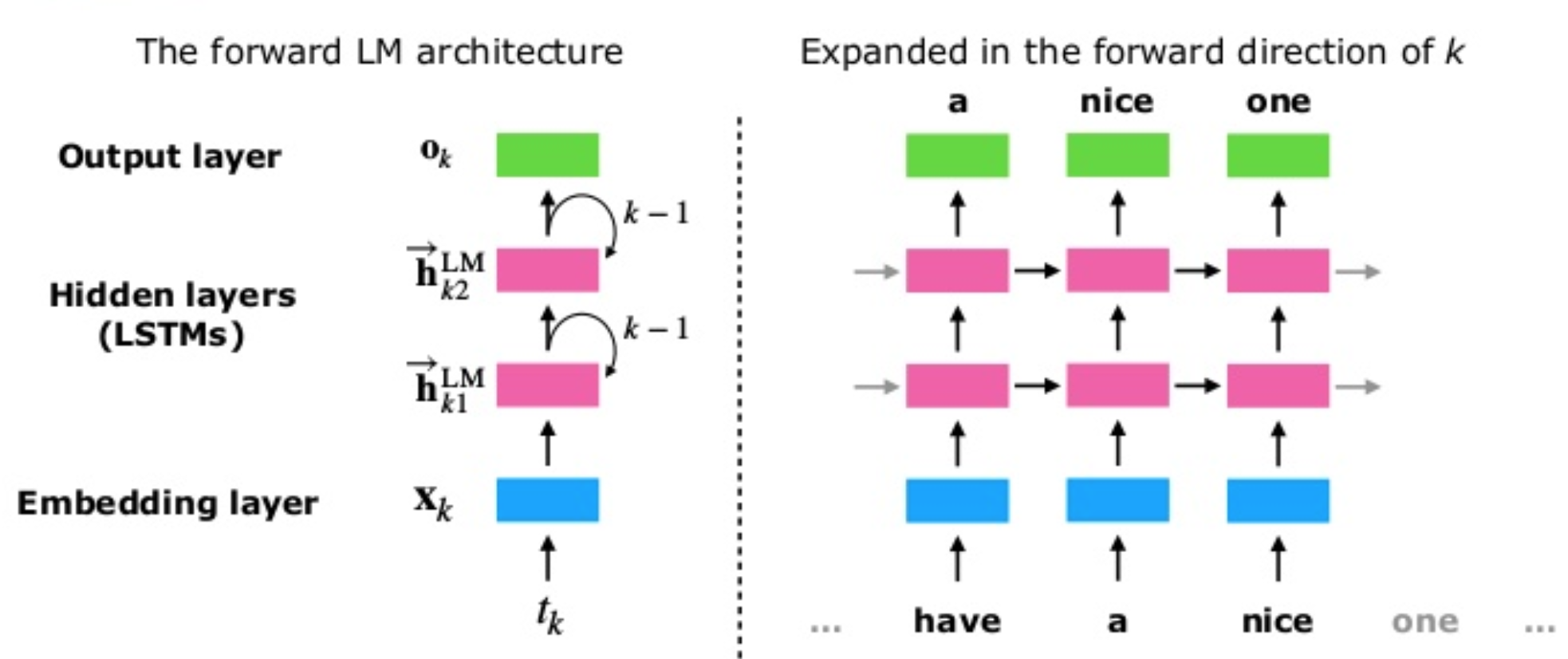
Image taken from Shuntaro Yada slides
Training $L$-layer LSTM forward and backward language mode generates \(2\ \times \ L\) different vector representations for each word, $L$ represents the number of stacked LSTMs, and each one outputs a vector.
Adding another vector representation of the word, trained on some external resources, or just a random embedding, we end up with \(2\ \times \ L + 1\) vectors that can be used to compute the context representation of every word.
The parameters for the token representations and the softmax layer are shared by the forward and backward language model, while the LSTM parameters (hidden state, gate, memory) are separate.
ELMo is a task-specific combination of the intermediate layer representations in a bidirectional Language Model (biLM). That is, given a pre-trained biLM and a supervised architecture for a target NLP task, the end task model learns a linear combination of the layer representations.
The language model described above is completely task-agnostic and is trained in an unsupervised manner.
Task-specific word representation
The second part of the model consists in using the hidden states generated by the LSTM for each token to compute a vector representation of each word, the detail here is that this is done in a specific context, with a given end task.
Concretely, in ELMo, each word representation is computed with a concatenation and a weighted sum:
\[ELMo_k = \gamma^{task} \sum_{j=0}^{L} s_j^{task} h_{k,j}^{LM}\]- the scalar parameter \(\gamma^{task}\) allows the task model to scale the entire ELMo vector
- \(s_j^{task}\) are softmax-normalized weights
- the indices \(k\) and \(j\) correspond to the index of the word and the index of the layer from which the hidden state is being extracted from.
For example, \(h_{k,j}\) is the output of the \(j\)-th LSTM for the word \(k\), \(s_j\) is the weight of \(h_{k,j}\) in computing the representation for \(k\).
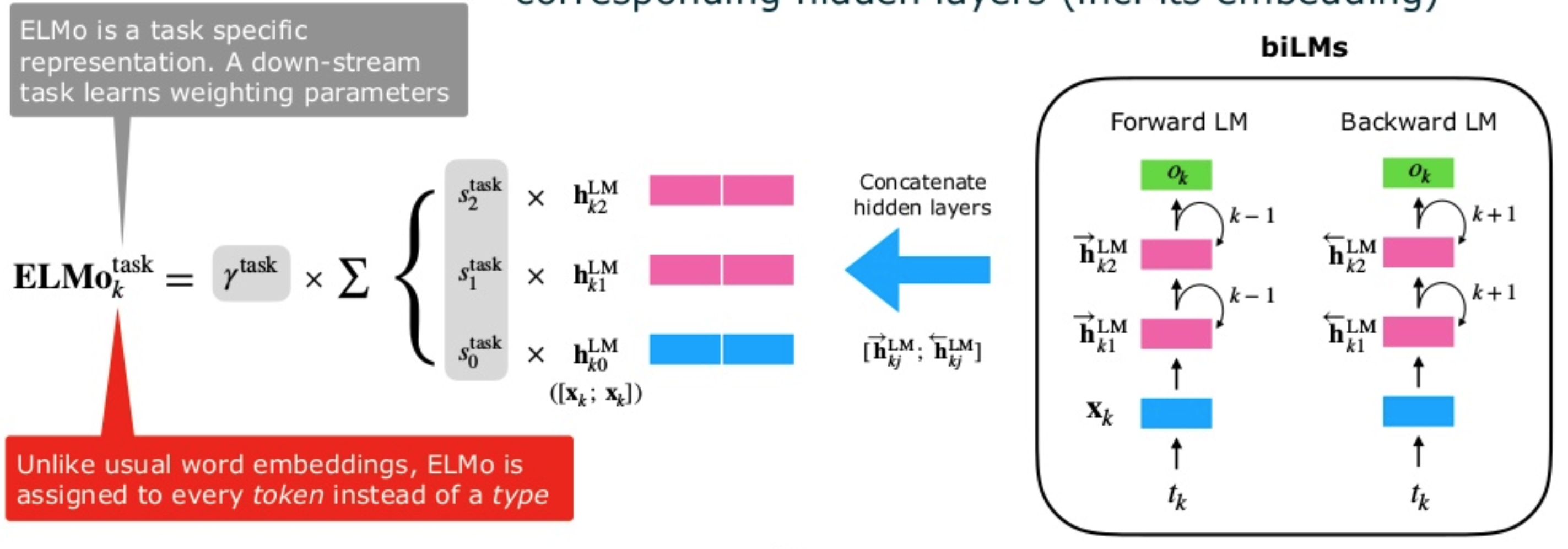
Image taken from Shuntaro Yada slides
In practice ELMo embeddings could replace existing word embeddings, the authors however recommend concatenating ELMos with context-independent word embeddings such as GloVe or fastText before inputting them into the task-specific model.
ELMo is flexible in the sense that it can be used with any model barely changing it, meaning it can work with existing systems or architectures.
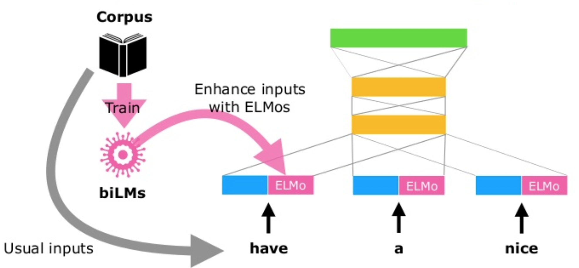
Image taken from Shuntaro Yada slides
In resume, ELMos train a multi-layer, bi-directional, LSTM-based language model, and extracts the hidden state of each layer for the input sequence of words. Then, they compute a weighted sum of those hidden states to obtain an embedding for each word. The weight of each hidden state is task-dependent and is learned during training for the end task.
Links
- ELMo code at AllenNLP github
- AllenNLP Models
- Video of the presentation of paper by Matthew Peters @ NAACL-HLT 2018
- Images were taken/adapted from Shuntaro Yada excellent slides
Contextual String Embeddings for Sequence Labelling (2018)
The authors propose a contextualised character-level word embedding which captures word meaning in context and therefore produces different embeddings for polysemous words depending on their context. It models words and context as sequences of characters, which aids in handling rare and misspelt words and captures subword structures such as prefixes and endings.
Character-level Language Model
Characters are the atomic units of the language model, allowing text to be treated as a sequence of characters passed to an LSTM which at each point in the sequence is trained to predict the next character.
The authors train a forward and a backward model character language model. Essentially the character-level language model is just ‘tuning’ the hidden states of the LSTM based on reading lots of sequences of characters.
The LSTM internal states will try to capture the probability distribution of characters given the previous characters (i.e., forward language model) and the upcoming characters (i.e., backward language model).
Extracting Word Representations
From this forward-backward LM, the authors concatenate the following hidden character states for each word:
-
from the fLM, we extract the output hidden state after the last character in the word. Since the fLM is trained to predict likely continuations of the sentence after this character, the hidden state encodes semantic-syntactic information of the sentence up to this point, including the word itself.
-
from the bLM, we extract the output hidden state before the word’s first character from the bLM to capture semantic-syntactic information from the end of the sentence to this character.
Both output hidden states are concatenated to form the final embedding and capture the semantic-syntactic information of the word itself as well as its surrounding context.
The image below illustrates how the embedding for the word Washington is generated, based on both character-level language models.
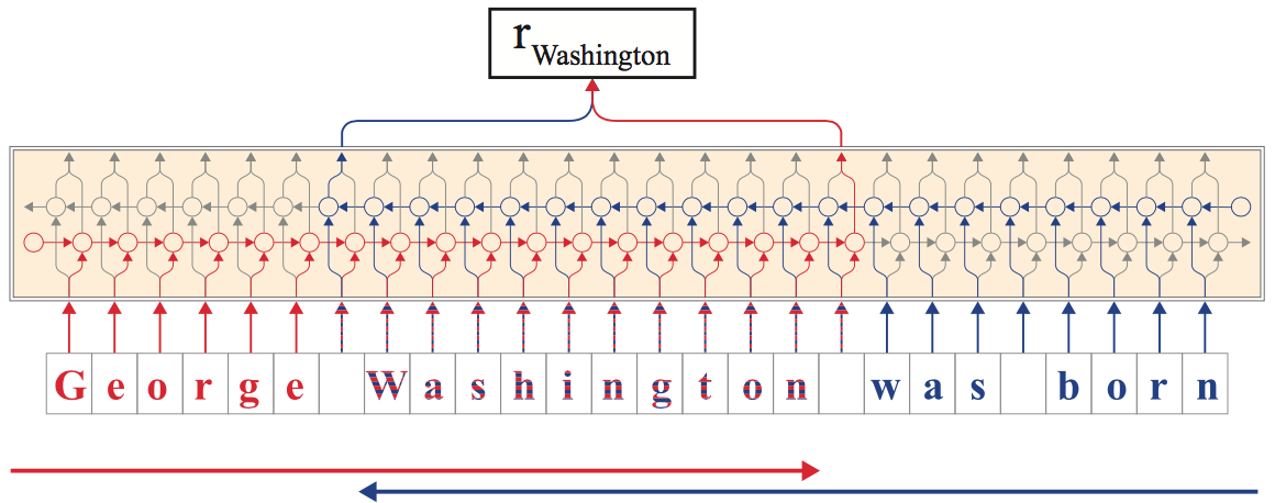
Image taken from "Contextual String Embeddings for Sequence Labelling (2018)"
The embeddings can then be used for other downstream tasks such as named-entity recognition. The embeddings generated from the character-level language models can also (and are in practice) be concatenated with word embeddings such as GloVe or fastText.
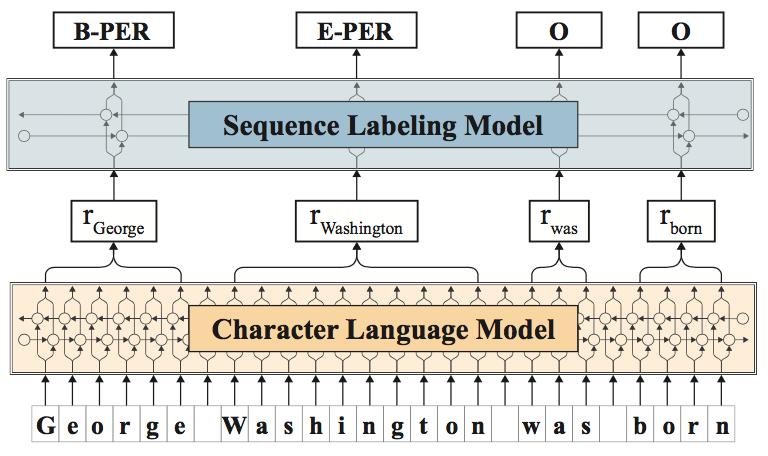
Image taken from "Contextual String Embeddings for Sequence Labelling (2018)"
In essence, this model first learns two character-based language models (i.e., forward and backward) using LSTMs. Then, an embedding for a given word is computed by feeding a word - character by character - into each of the language models and keeping the two last states (i.e., last character and first character) as two-word vectors, these are then concatenated.
In the experiments described in the paper, the authors concatenated the word vector generated before with yet another word vector from fastText and then apply a Neural NER architecture for several sequence labelling tasks, e.g.: NER, chunking, PoS-tagging.
Links
BERT: Pre-training of Deep Bidirectional Transformers for Language Understanding (2018)
BERT, or Bidirectional Encoder Representations from Transformers, is essentially a new method of training language models.
Pre-trained word representations, as seen in this blog post, can be context-free (i.e., word2vec, GloVe, fastText), meaning that a single word representation is generated for each word in the vocabulary, or can also be contextual (i.e., ELMo and Flair), on which the word representation depends on the context where that word occurs, meaning that the same word in different contexts can have different representations.
Contextual representations can further be unidirectional or bidirectional. Note, even if a language model is trained forward or backward, is still considered unidirectional since the prediction of future words (or characters) is only based on past seen data.
In the sentence: “The cat sits on the mat”, the unidirectional representation of “sits” is only based on “The cat” but not on “on the mat”. Previous works train two representations for each word (or character), one left-to-right and one right-to-left, and then concatenate them together to have a single representation for whatever downstream task.
BERT represents “sits” using both its left and right context — “The cat xxx on the mat” based on a simple approach, masking out 15% of the words in the input, running the entire sequence through a multi-layer bidirectional Transformer encoder, and then predict only the masked words.
Multi-layer bidirectional Transformer encoder
The Multi-layer bidirectional Transformer aka Transformer was first introduced in the Attention is All You Need paper. It follows the encoder-decoder architecture of machine translation models, but it replaces the RNNs with a different network architecture.
The Transformer tries to learn the dependencies, typically encoded by the hidden states of an RNN, using just an Attention Mechanism. RNNs handle dependencies by being stateful, i.e., the current state encodes the information they needed to decide on how to process subsequent tokens.
This means that RNNs need to keep the state while processing all the words, and this becomes a problem for long-range dependencies between words. The attention mechanism has somehow mitigated this problem but it still remains an obstacle to high-performance machine translation.
The Transformer tries to directly learn these dependencies using the attention mechanism only and it also learns intra-dependencies between the input tokens, and between output tokens. This is done by relying on a key component, the Multi-Head Attention block, which has an attention mechanism defined by the authors as the Scaled Dot-Product Attention.
Image taken from "Attention Is All You Need"
To improve the expressiveness of the model, instead of computing a single attention pass over the values, the Multi-Head Attention computes multiple attention-weighted sums, i.e., it uses several attention layers stacked together with different linear transformations of the same input.
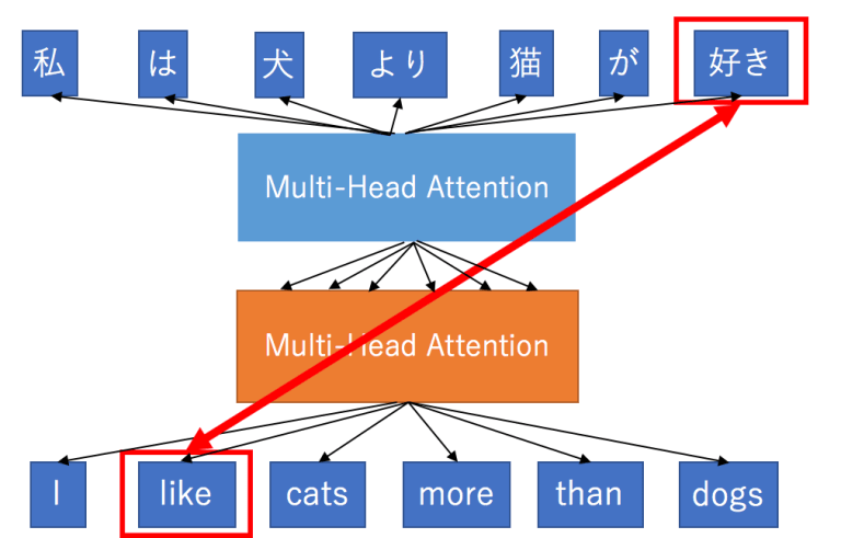
Image taken from http://mlexplained.com/2017/12/29/attention-is-all-you-need-explained/
The main key feature of the Transformer is therefore that instead of encoding dependencies in the hidden state, directly expresses them by attending to various parts of the input.
The Transformer in an encoder and a decoder scenario
Image taken from "Attention Is All You Need"
This is just a very brief explanation of what the Transformer is, please check the original paper and following links for a more detailed description:
- http://mlexplained.com/2017/12/29/attention-is-all-you-need-explained/
- https://ai.googleblog.com/2017/08/transformer-novel-neural-network.html
- http://nlp.seas.harvard.edu/2018/04/03/attention.html
Masked Language Model
BERT uses the Transformer encoder to learn a language model.
The input to the Transformer is a sequence of tokens, which are passed to an embeddeding layer and then processed by the Transformer network. The output is a sequence of vectors, in which each vector corresponds to an input token.
Image taken from https://www.lyrn.ai/2018/11/07/explained-bert-state-of-the-art-language-model-for-nlp/
As explained above this language model is what one could consider a bi-directional model, but some defend that you should be instead called non-directional.
The bi-directional/non-directional property in BERT comes from masking 15% of the words in a sentence and forcing the model to learn how to use information from the entire sentence to deduce what words are missing.
The original Transformer is adapted so that the loss function only considers the prediction of masked words and ignores the prediction of the non-masked words. The prediction of the output words requires:
- Adding a classification layer on top of the encoder output.
- An embedding matrix, transforming the output vectors into the vocabulary dimension.
- Calculating the probability of each word in the vocabulary with softmax.
Image taken from https://www.lyrn.ai/2018/11/07/explained-bert-state-of-the-art-language-model-for-nlp/
BRET is also trained in a Next Sentence Prediction (NSP), in which the model receives pairs of sentences as input and has to learn to predict if the second sentence in the pair is the subsequent sentence in the original document or not.
To use BERT for a sequence labelling task, for instance, a NER model, this model can be trained by feeding the output vector of each token into a classification layer that predicts the NER label.
Links
- Open Sourcing BERT: State-of-the-Art Pre-training for Natural Language Processing
- https://github.com/google-research/bert
- BERT – State of the Art Language Model for NLP (www.lyrn.ai)
- Reddit: Pre-training of Deep Bidirectional Transformers for Language Understanding
- The Illustrated BERT, ELMo, and co. (How NLP Cracked Transfer Learning)
Summary
In a time span of about 10 years, Word Embeddings revolutionised the way almost all NLP tasks can be solved, essentially by replacing the feature extraction/engineering with embeddings which are then fed as input to different neural network architectures.
The most popular models started around 2013 with the word2vec package, but a few years before there were already some results in the famous work of Collobert et, al 2011 Natural Language Processing (Almost) from Scratch which I did not mention above.
Nevertheless, these techniques, along with GloVe and fastText, generate static embeddings which are unable to capture polysemy, i.e the same word having different meanings. Typically these techniques generate a matrix that can be plugged into the current neural network model and is used to perform a lookup operation, mapping a word to a vector.
Recently other methods which rely on language models and also provide a mechanism of having embeddings computed dynamically as a sentence or a sequence of tokens is being processed.
References
- Efficient Estimation of Word Representations in Vector Space (2013)
- McCormick, C. (2016, April 19). Word2Vec Tutorial - The Skip-Gram Model.
- McCormick, C. (2017, January 11). Word2Vec Tutorial Part 2 - Negative Sampling.
- word2vec Parameter Learning Explained, Xin Rong
- GloVe: Global Vectors for Word Representation (2014)
- Enriching Word Vectors with Subword Information (2017)
- ELMo: Deep contextualized word representations (2018)__
- Contextual String Embeddings for Sequence Labelling__ (2018)
- BERT: Pre-training of Deep Bidirectional Transformers for Language Understanding (2018)
- https://ai.googleblog.com/2017/08/transformer-novel-neural-network.html
- http://nlp.seas.harvard.edu/2018/04/03/attention.html
- Open Sourcing BERT: State-of-the-Art Pre-training for Natural Language Processing
word-embeddings language-models neural-networks 