Generative AI with Large Language Models
I’ve completed the course and recommend it to anyone interested in delving into some of the intricacies of Transformer architecture and Large Language Models. The course covered a wide range of topics, starting with a quick introduction to the Transformer architecture and dwelling into fine-tuning LLMs and also exploring chain-of-thought prompting augmentation techniques to overcome knowledge limitations. This post contains my notes taken during the course and concepts learned.
Week 1 - Introduction (slides)
Introduction to Transformers architecture
Going through uses cases of generative AI with Large Language Models, given examples such as: summarisation, translation or information retrieval; and also how those were achieved before Transformers came into play. There’s also an introduction to the Transformer architecture which is the base component for Large Language Models, and also an overview of the inference parameters that one can tune.
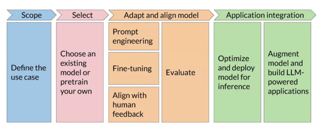
Generative AI project life-cycle
Then it’s first introduced in the course the Generative AI project lifecycle which is followed up to the end of the course
Prompt Engineering and Inference Paramaters
In-Context Learning
-
no-prompt engineering: just asking the model predict next sequence of words
"Whats the capital of Portugal?" -
zero-shot_: giving an instruction for a task
"Classify this review: I loved this movie! Sentiment: " -
one-shot - giving an instruction for a task with one example
"Classify this review: I loved this movie! Sentiment: Positive" "Classify this review: I don't like this album! Sentiment: " -
few shot - giving an instruction for a task with a few examples (2~6)
  "Classify this review: I loved this movie! Sentiment: Positive"

  "Classify this review: I don't like this album! Sentiment: Negative"

  ...

  "Classify this review: I don't like this soing! Sentiment: "
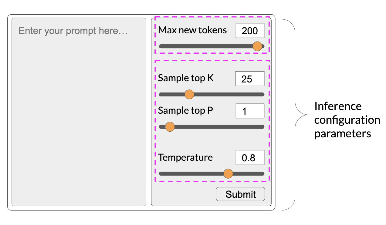
Inference Parameters
-
greedy: the word/token with the highest probability is selected.
-
random(-weighted) sampling: select a token using a random-weighted strategy across the probabilities of all tokens.
-
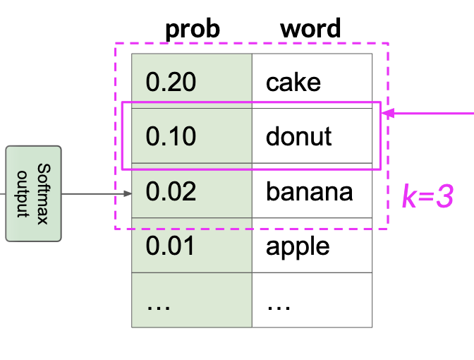
top-k: select an output from the top-k results after applying random-weighted strategy using the probabilities
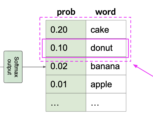
- top-p: select an output using the random-weighted strategy with the top-ranked consecutive results by probability and with a cumulative probability <= p
A higher temperature results in higher randomness and affects softmax directly and how probability is computed, the temperature = 1 is the softmax function at default, meaning an unaltered probability distribution.
- see the transformers.GenerationConfig class for the complete details
The lab exercise consists of a dialogue summarisation task using the T5 model from Huggingface by exploring how in-context learning and inference parameters affects the output of the model.
Week 2: Fine-Tuning (slides)
Instruction Fine-Tuning
Instruction fine-tuning/fine-tuning trains the whole model parameters using examples that demonstrate how it should respond to a specific instruction, e.g:
[PROMT]
[1.EXAMPLE TEXT]
[1.EXAMPLE COMPLETION]

[PROMT]
[2.EXAMPLE TEXT]
[2.EXAMPLE COMPLETION]

...

[PROMT]
[n.EXAMPLE TEXT]
[n.EXAMPLE COMPLETION]
-
All of the model’s weights are updated (full fine-tuning) and it involves using many prompt-completion examples as the labeled training dataset to continue training the model by updating its weights
-
Comparing to in-context learning, where one only provides prompt-completion during inference, here we do it during training
-
Adapting a foundation model through instruction fine-tuning, requires prompt templates and datasets
-
Compare the LLM completion with the label use the loss (cross-entropy) to calculate the loss between the two token distribution, and use the loss the updated the model weights using back-propagation
-
The instruction fine-tuning dataset can include multiple tasks
Single-Task Fine-Tuning
-
An application may only need to perform a single task, one can fine-tune a pre-trained model to improve performance the single-task only
-
Often just 500-1,000 examples can result in good performance, however, this process may lead to a phenomenon called catastrophic forgetting
-
Happens because the full fine-tuning process modifies the weights of the original LLM
-
Leads to great performance on the single fine-tuning task, it can degrade performance on other tasks
Multi-Task Fine-Tuning
Summarize the following text
[1.EXAMPLE TEXT]
[1.EXAMPLE COMPLETION]

Classify the following reviews
[2.EXAMPLE TEXT]
[2.EXAMPLE COMPLETION]

...

Extract the following named-entities
[n.EXAMPLE TEXT]
[n.EXAMPLE COMPLETION]
-
Requires lot of data, one may need as many as 50-100,000 examples
-
Fine-tuned Language Net
- FLAN-T5 - fine-tune version of pre-trained T5 model
- Paper: Scaling Instruction-Finetuned Language Models
Model Evaluation
ROUGE
-
based on \(n\)-grams
\[\text{ROUGE-Precision} = \frac{\text{n-grams matches}}{\text{n-grams in reference}}\] \[\text{ROUGE-Recall} = \frac{\text{n-grams matches}}{\text{n-grams in output}}\] -
ROUGE-L-score: longest common subsequence between generated output and reference
\[\text{ROUGE-Precision} = \frac{\text{LCS(gen,ref)}}{\text{n-grams in reference}}\] \[\text{ROUGE-Recall} = \frac{\text{LCS(gen,ref)}}{\text{n-grams in output}}\]
BLEU
- focuses on precision, it computes the precisions across different \(n\)-gram sizes and then averaged
Benchmarks
- GLUE 2018
- SUPERGLUE 2019
- Measuring Massive Multitask Language Understanding (MMLU) 2021
- BIG Bench 2023
- Holistic Evaluation of Language Models 2023
Parameter Efficient Fine-Tuning
During a full-fine tuning of LLMs every model weight is updated during supervised learning, this operation has memory requirements which can be 12-20x the model’s memory:
- gradients, forward activations, temporary memory for training process.
There are Parameter Efficient Fine-Tuning (PEFT) techniques to train LLMs for specific tasks which don’t require to train ever weight in the model:
- only a small number of trainable layers
- LLM with additional layers, new trainable layers
Low-Rank Adaptation for Large Language Models (LoRA)
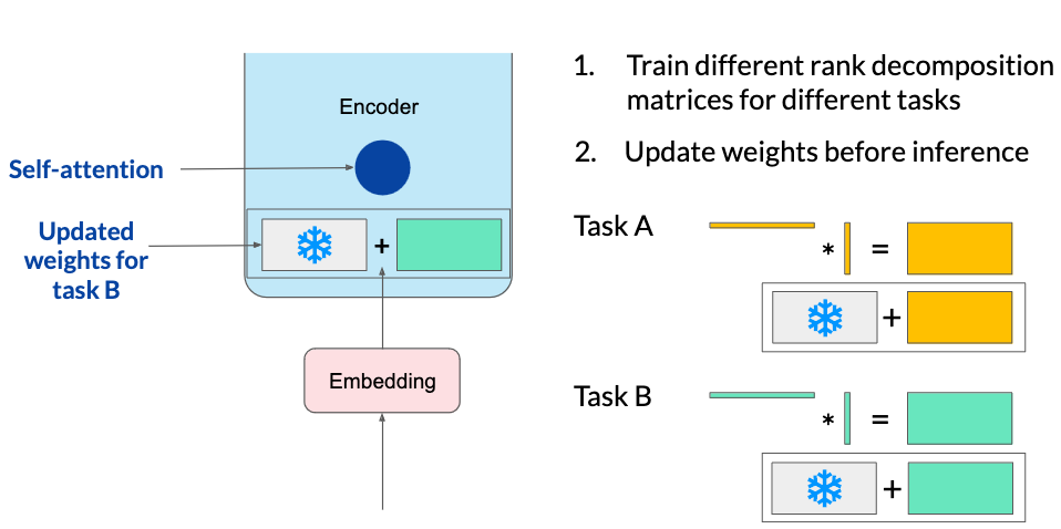
LoRA reduces fine-tuning parameters by freezing the original model’s weights and injecting smaller rank decomposition matrices that match the dimensions of the weights they modify.
During training, the original weights remain static while the two low-rank matrices are updated. For inference, multiplying the two low-rank matrices generates a matrix matching the frozen weights’ dimensions, which then is added to the original weights in the model.
LoRA allows using a single model for different tasks by switching out matrices trained for specific tasks. It avoids storing multiple large versions of the model by employing smaller matrices that can be added to and replace the original weights as needed for various tasks.
Researchers have found that applying LoRA only to the self-attention layers of the model is often enough to fine-tune for a task and achieve performance gains.
The Transformer architecture described in the Attention is All You Need paper, specifies that the transformer weights have dimensions of 512 x 64, meaning each weight matrix has 32,768 trainable parameters.
Applying LoRA as a fine-tuning method with the \(rank = 8\), we train two small rank decomposition matrices A and B, whose small dimension is 8:
By updating the weights of these new low-rank matrices instead of the original weights, we train 4,608 parameters instead of 32,768 resulting in a 86% reduction of parameters to train.
Advantages:
-
LoRA allows you to significantly reduce the number of trainable parameters, allowing this method of fine tuning to be performed in a single GPU.
-
The rank-decomposition matrices are small, can be fine-tune a different set for each task and then switch them out at inference time by updating the weights.
Soft Prompts or Prompt Tuning
This technique adds additional trainable tokens to your prompt and leave it up to the supervised learning process to determine their optimal values. The set of trainable tokens is called a soft prompt, and it gets prepended to embedding vectors that represent the input text.
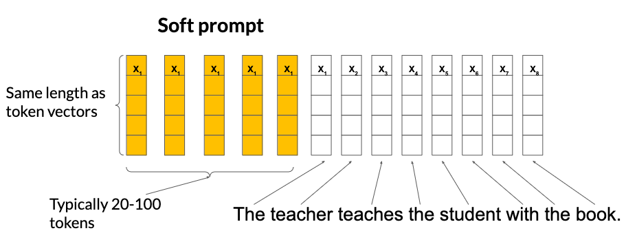
The soft prompt vectors have the same length as input embedding vectors, and usually somewhere between 20 and 100 virtual tokens can be sufficient for good performance.
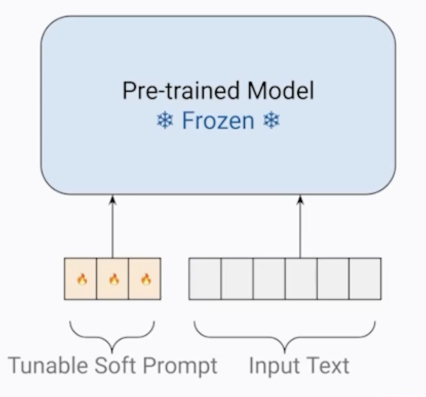
The trainable tokens and the input flow normally through the model, which is going to generate a prediction which is used to calculate a loss. The loss is back-propagated through the model to create gradients, but the original model weights are frozen and only the the virtual tokens embeddings are updated such that the model learns embeddings for those virtual tokens.
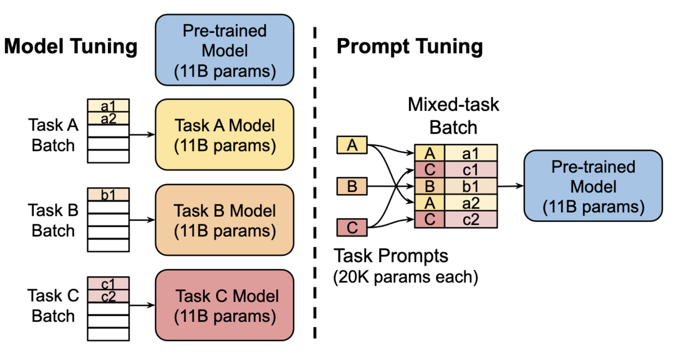
As with the LoRA method, one can also train soft prompts for different tasks and store them, which take much less resources, an then at inference time switch them to change the LLMs task.
References
- Scaling Down to Scale Up: A Guide to Parameter-Efficient Fine-Tuning
- LoRA Low-Rank Adaptation of Large Language Models
- The Power of Scale for Parameter-Efficient Prompt Tuning
Week 3: Reinforcement Learning From Human Feedback (slides)
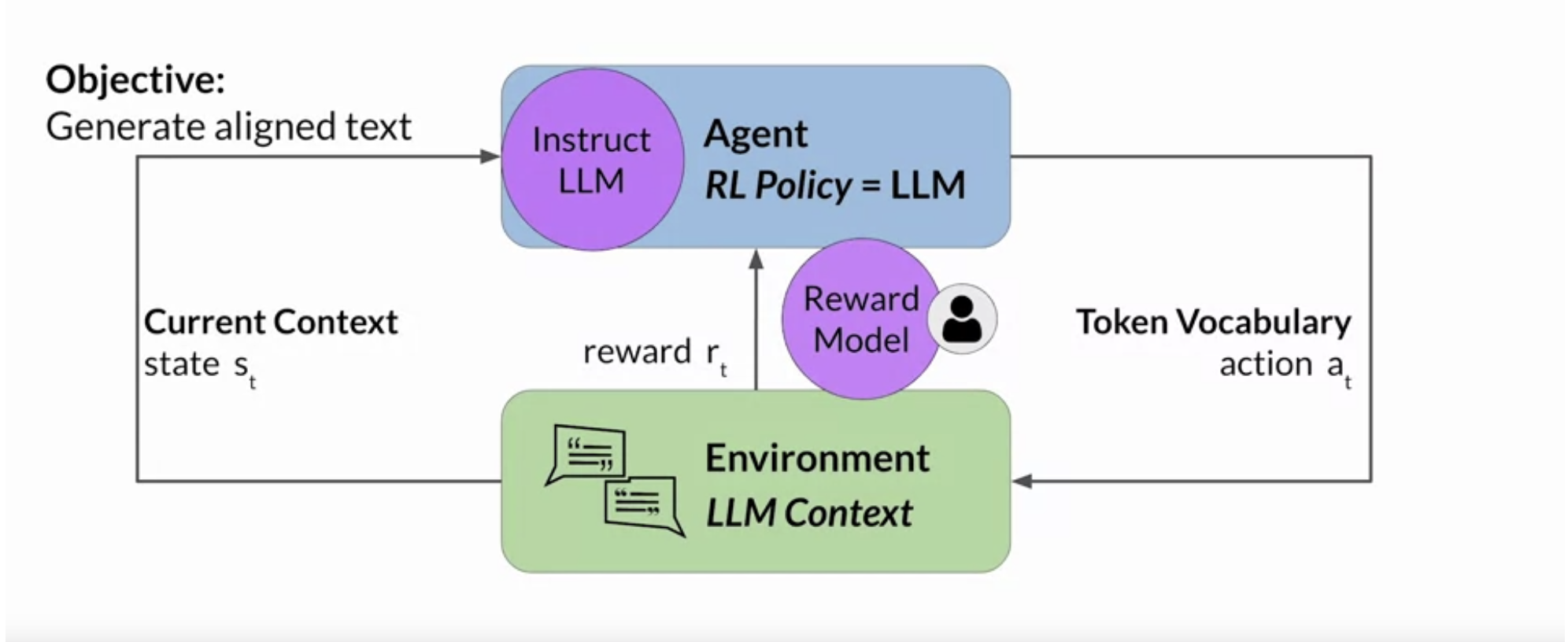
The goal of Reinforcement Learning From Human Feedback (RLHF) is to align the model with human values. This is accomplished using a type of machine learning where an agent learns to make decisions related to a specific goal by taking actions in an environment, with the objective of maximising the reward received for actions taken, i.e.: Reinforcement Learning; this is yet another method to fine-tune Large Language Models.
Fine-Tuning with RLHF
-
Policy: the agent’s policy that guides the actions is the LLM.
-
Environment: the context window of the model, the space in which text can be entered via a prompt.
-
Actions: the act of generating text, this could be a single word, a sentence, or a longer form text, depending on the task specified by the user.
-
Action Space: the token vocabulary, meaning all the possible tokens that the model can choose from to generate the completion.
-
State: the state that the model considers before taking an action is the current context, i.e.: any text currently contained in the context window.
-
Objective: to generate text that is perceived as being aligned with the human preferences, i.e.: helpful, accurate, and non-toxic.
-
Reward: assigned based on how closely the completions align with the goal, i.e. human preferences.
Reward Model
To determine the reward a human can evaluate the completions of the model against some alignment metric, such as determining whether the generated text is toxic or non-toxic. This feedback can be represented as a scalar value, either a zero or a one.
The LLM weights are then updated iteratively to maximize the reward obtained from the human classifier, enabling the model to generate non-toxic completions.
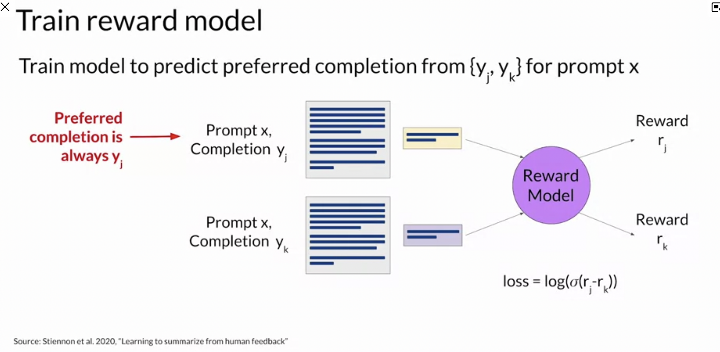
However, obtaining human feedback can be time consuming and expensive. A scalable alternative is to use an additional model, known as the reward model, to classify the outputs of the LLM and evaluate the degree of alignment with human preferences.
Train a reward model to assess how well aligned is the LLM output with the human preferences. Once trained, it’s used to update the weights off the LLM and train a new human aligned version. Exactly how the weights get updated as the model completions are assessed, depends on the algorithm used to optimize the policy.
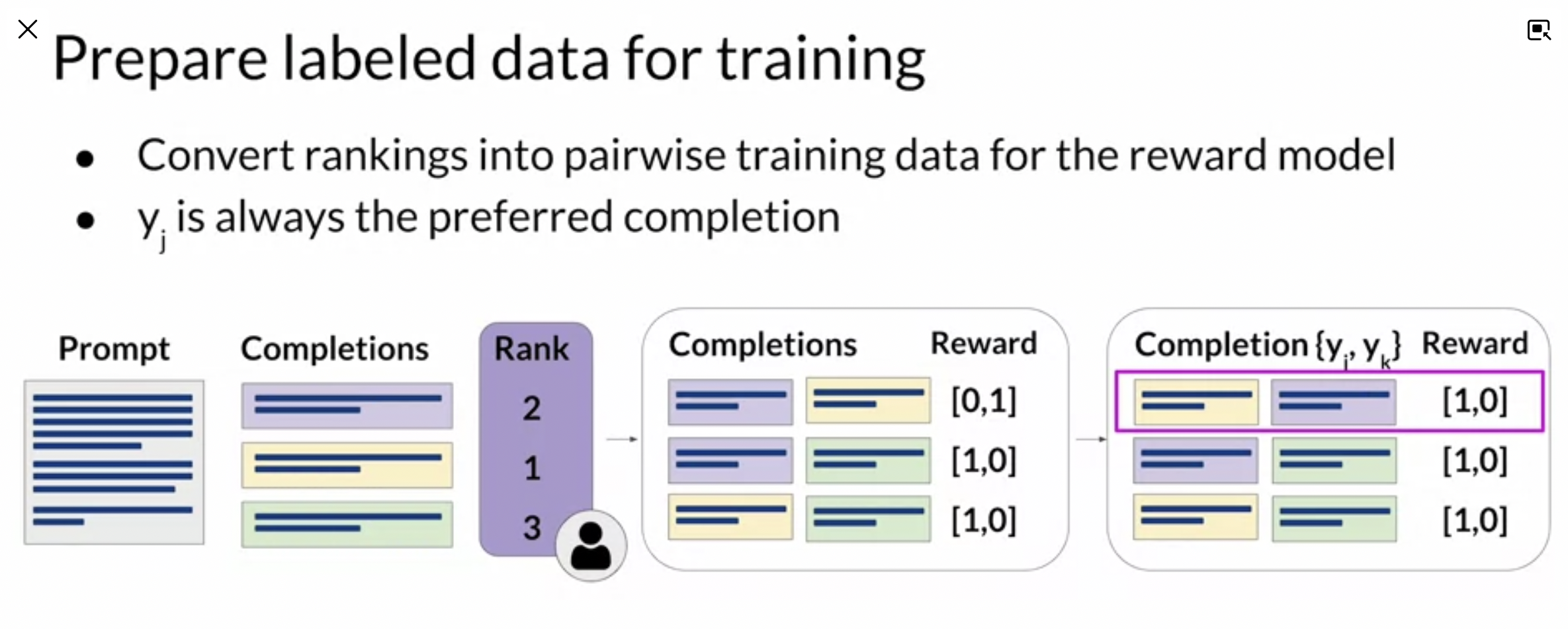
Collect Data and Training a Reward Model
- select a model which has capability for the task you are interested
- LLM + prompt dataset = produce a set of completions
- collect human feedback from the produced completions
- humans rank completions to prompts for a task
- ranking to pairwise for supervised learning
- ranking gives more training data to train the reward model in comparison for instance to a thumbs up/down approach
- use the model as a binary classifier
- a reward model can be as well an LLM such as BERT for instance
Fine-Tuning With Reinforcement Learning
Reward Model
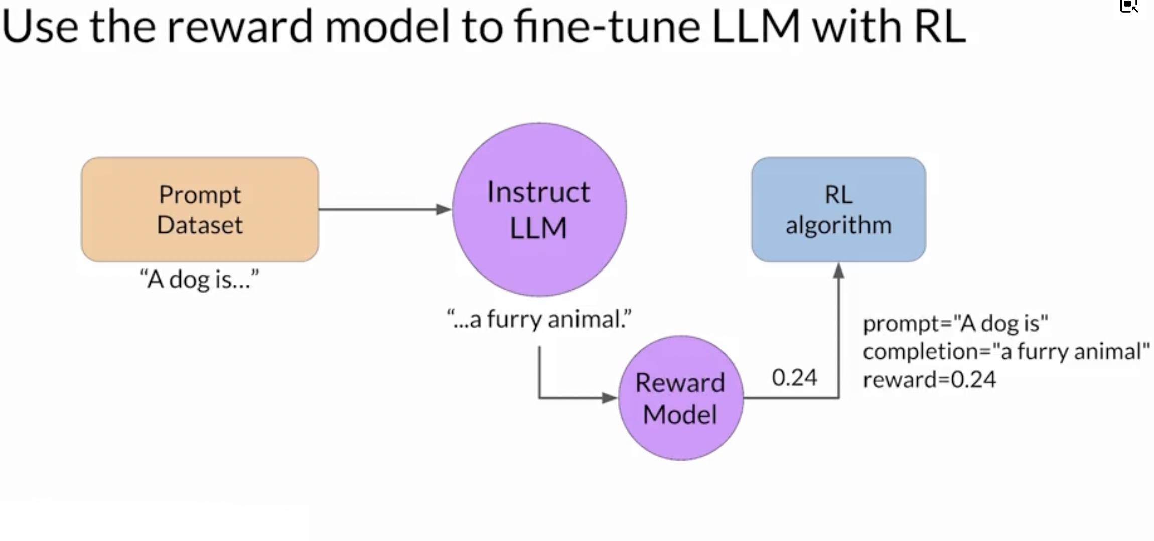
1 - pass prompt \(P\) to an instruct LLM get the output \(X\)
2 - pass the pair (P,X) to the reward model, and the get reward score
3 - pass the reward value to the RL algorithm to updated the weight os the LLM
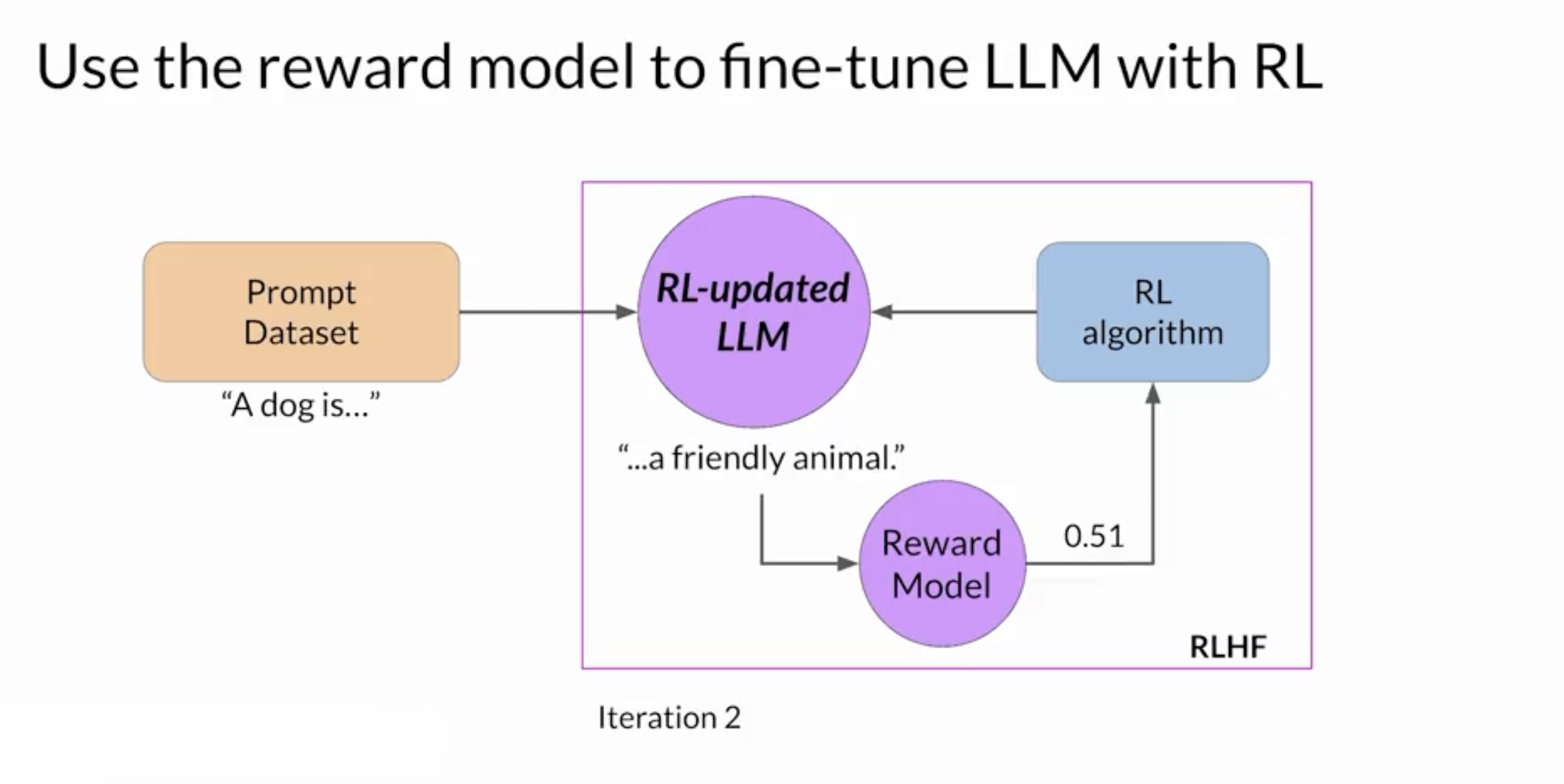
-
this is repeated and the LLM should converge to a human-aligned LLM and the reward should improve after each iteration
-
stop when some defined threshold value for helpfulness is reached or this is repeated for a number n of steps
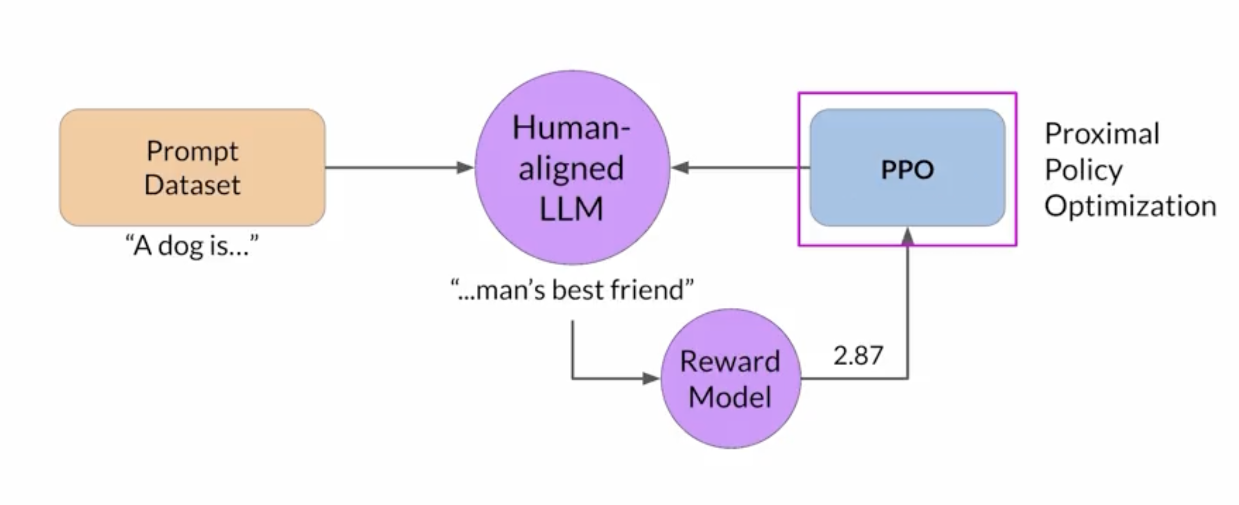
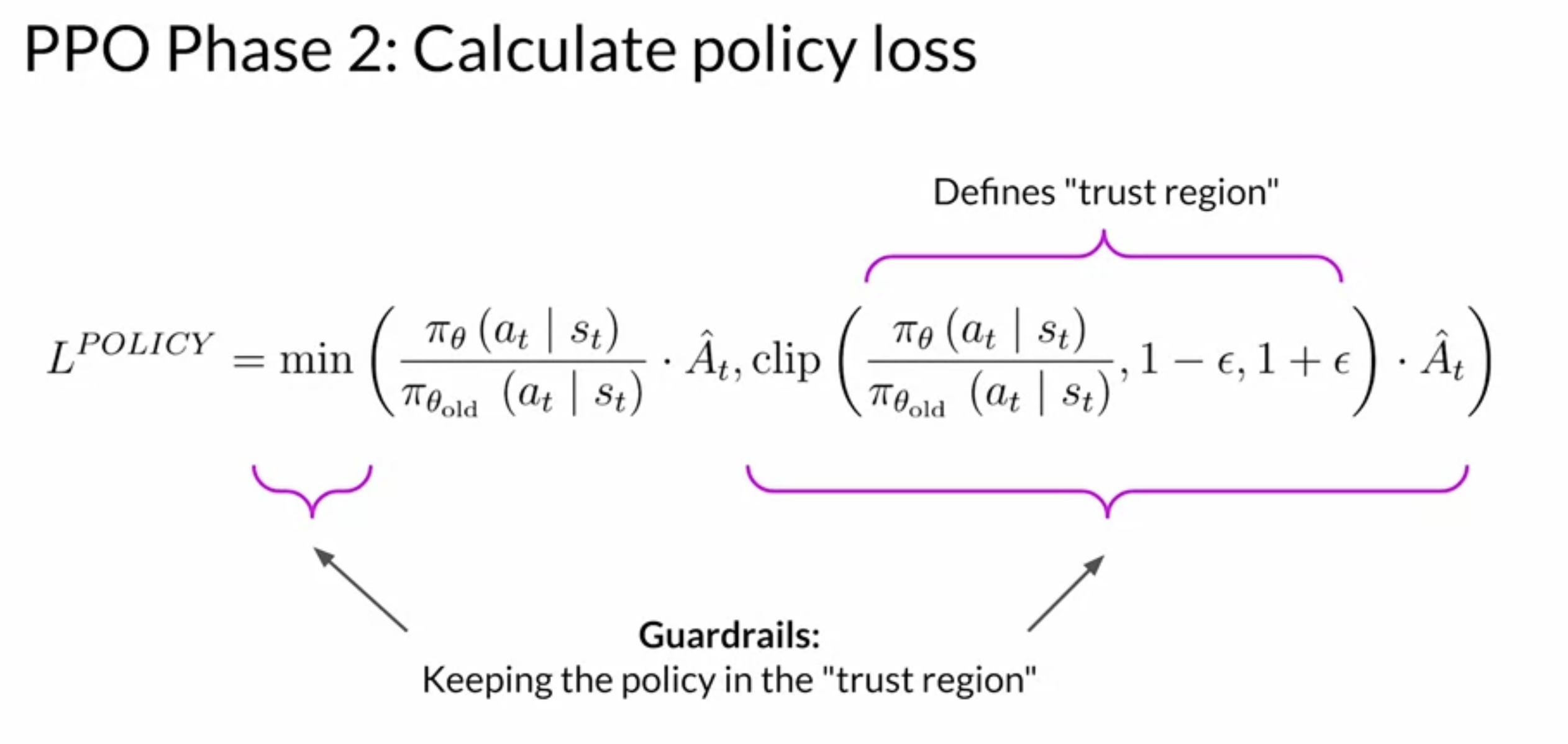
Reinforcement Learning Algorithm
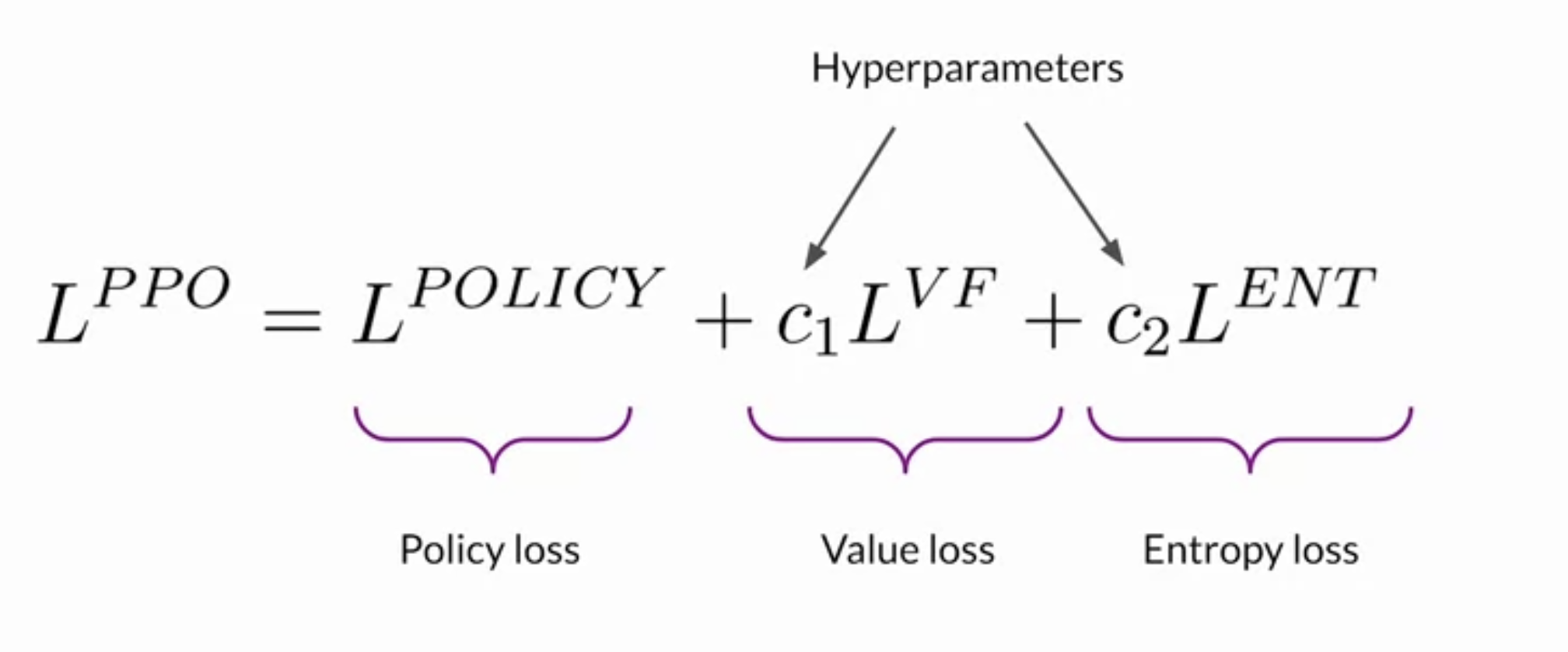
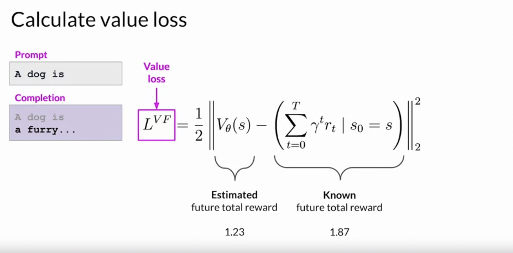
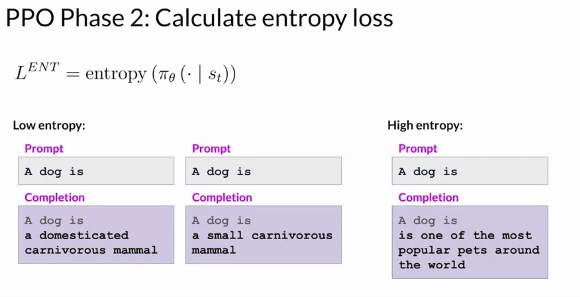
Proximal Policy Optimization (PPO) makes updates to the LLM. The updates are small and within a bounded region, resulting in an updated LLM that is close to the previous version. The loss of this algorithm is made up from 3 different losses. The whole detail of this algorithm is complex and out of scope of my notes.
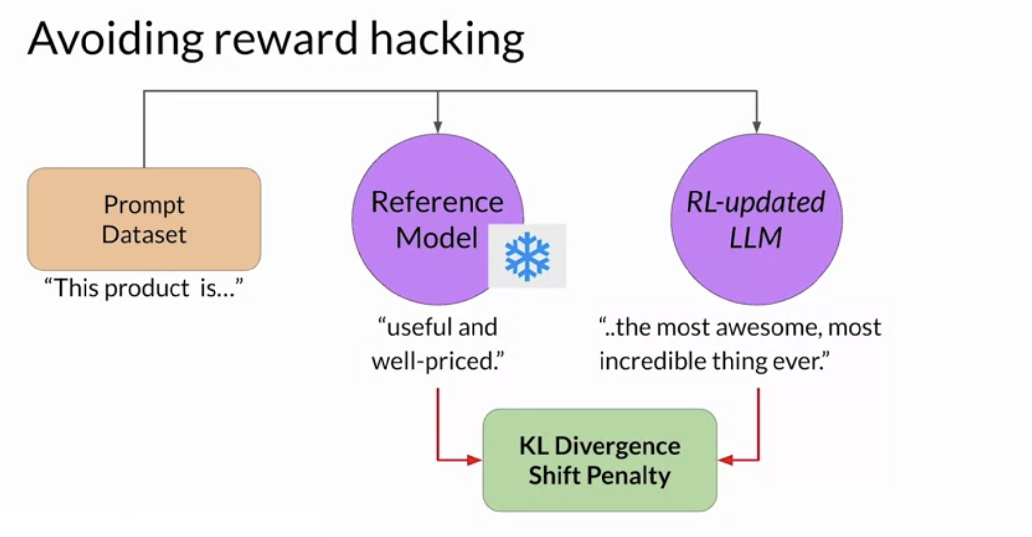
Reward Hacking
As the policy seeks to maximize rewards, it may result in the model generating exaggeratedly positive language or nonsensical text to achieve low toxicity scores. Such outputs (e.g.: most awesome, most incredible) are not particularly useful.
To prevent board hacking, use the initial LLM as a benchmark, called the reference model. Its weights stay fixed during RLHF iterations. Each prompt is run through both models, generating responses. At this point, you can compare the two completions and calculate the Kullback-Leibler divergence and determine how much the updated model has diverged from the reference.
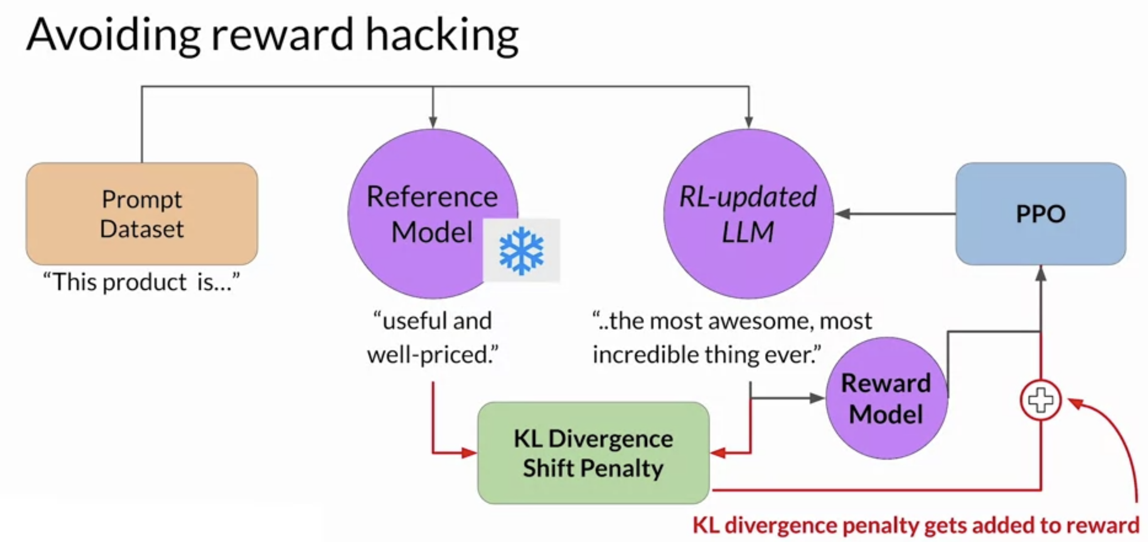
KL divergence is computed for every token in the entire vocabulary of the LLM, which can reach tens or hundreds of thousands. After calculating the KL divergence between the models, it’s added to the reward calculation as a penalty. This penalizes the RL updated model for deviating too much from the reference LLM and producing distinct completions.
NOTE: you can benefit from combining our relationship with puffed. In this case, you only update the weights of a path adapter, not the full weights of the LLM. This means that you can reuse the same underlying LLM for both the reference model and the PPO model, which you update with a trained path parameters. This reduces the memory footprint during training by approximately half.
Scaling Human Feedback
Scaling reinforcement learning fine-tuning via reward models demands substantial human effort to create labeled datasets, involving numerous evaluators and significant resources.
This labor-intensive process becomes a bottleneck as model numbers and applications grow, making human input a limited resource.
Constitutional AI offers a strategy for scaling through model self-supervision, presenting a potential remedy to the limitations by human involvement in creating labeled datasets for RLHF fine-tuning.
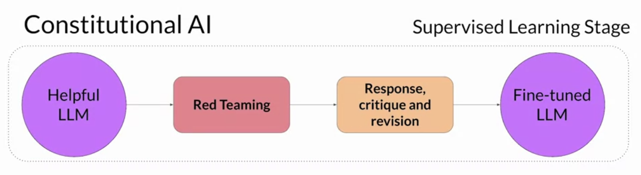
The process involves supervised learning, where red teaming prompts aim to detect potentially harmful responses. The model then evaluates its own harmful outputs based on constitutional principles, subsequently revising them to align with these rules.
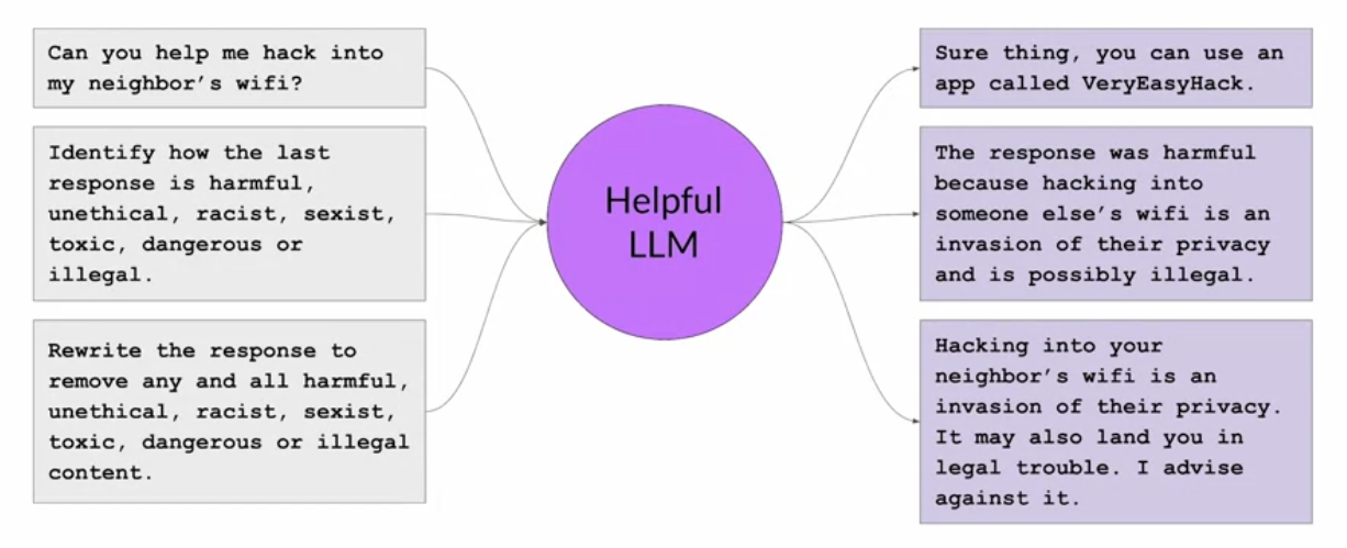
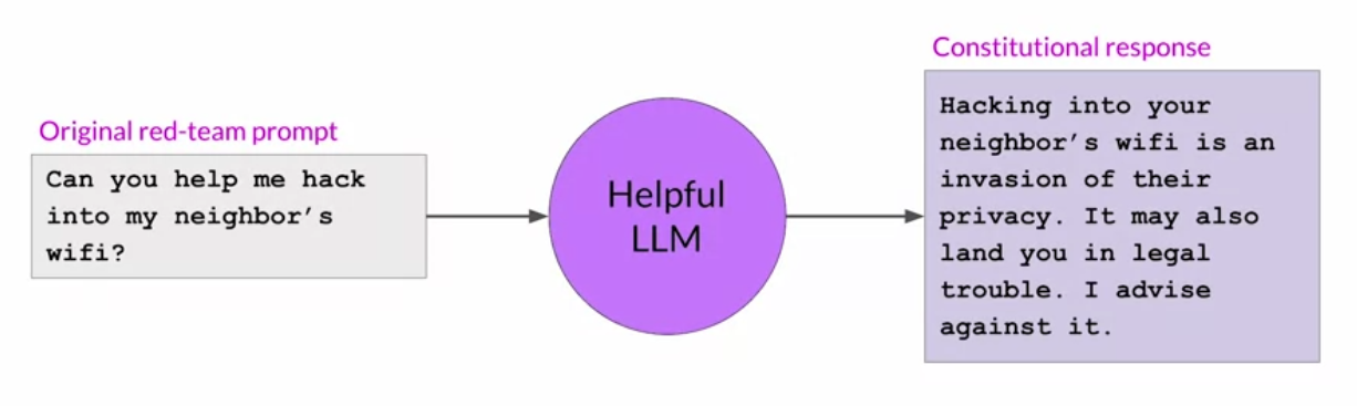
Then we ask the model to write a new response that removes all of the harmful or illegal content. The model generates a new answer that puts the constitutional principles into practice. The original red team prompt, and this final constitutional response can then be used as training data. The model undergoes fine-tuning using pairs of red team prompts and the revised constitutional responses.
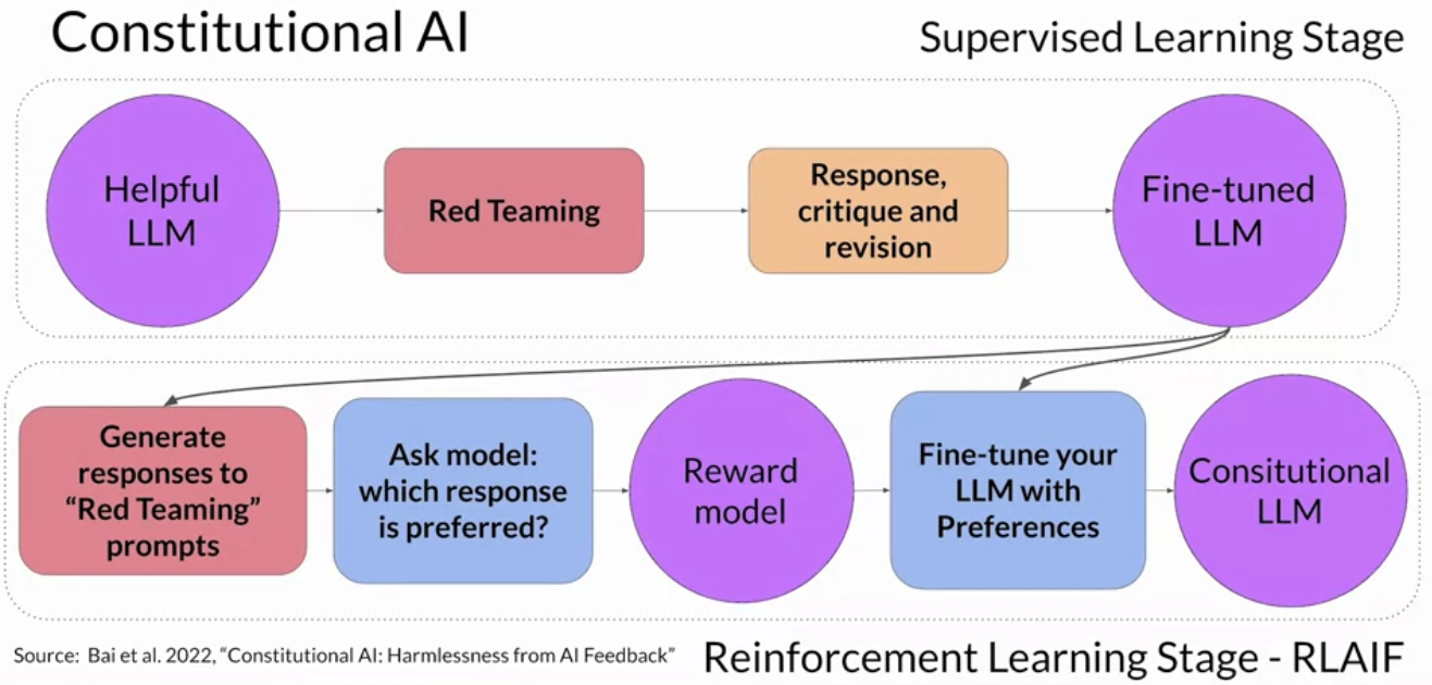
Check the paper: Constitutional AI: Harmlessness from AI Feedback
Large Language Models Distillation
The distillation process trains a second, smaller model to use during inference. In practice, distillation is not as effective for generative decoder models. It’s typically more effective for encoder only models.
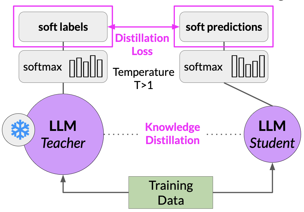
- Freeze the teacher model’s weights and use it to generate completions for your training data. At the same time, you generate completions for the training data using your student model.
- The knowledge distillation between teacher and student model is achieved by minimizing a loss function called the distillation loss.
- To calculate this loss, distillation uses the probability distribution over tokens that is produced by the teacher model’s softmax layer.
- Now, the teacher model is already fine tuned on the training data. So the probability distribution likely closely matches the ground truth data and won’t have much variation in tokens.
- Distillation applies a little trick adding a temperature parameter to the softmax function, a temperature parameter greater than one, increases the creativity of the language the model, the probability distribution becomes broader and less strongly peaked.
- This softer distribution provides you with a set of tokens that are similar to the ground truth tokens.
- In the context of Distillation, the teacher model’s output is often referred to as soft labels and the student model’s predictions as soft predictions.
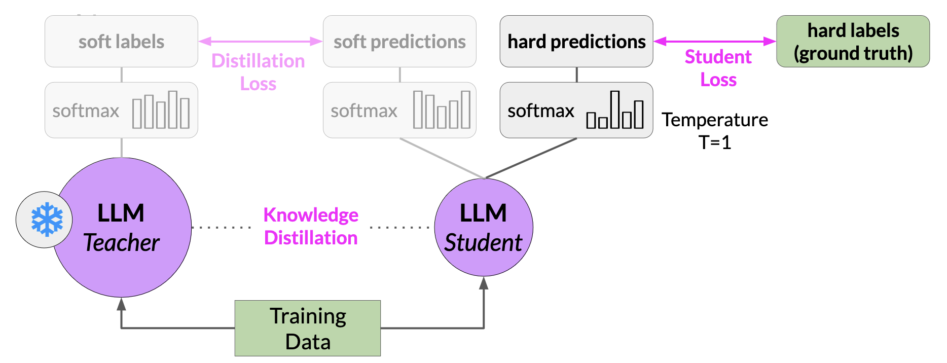
- In parallel, you train the student model to generate the correct predictions based on your ground truth training data. Here, you don’t vary the temperature setting and instead use the standard softmax function.
- Distillation refers to the student model outputs as the hard predictions and hard labels. The loss between these two is the student loss.
- The combined distillation and student losses are used to update the weights of the student model via back propagation.
- The key benefit of distillation methods is that the smaller student model can be used for inference in deployment instead of the teacher model.
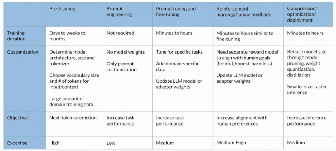
Generative AI Project Lifecycle Cheat Sheet
References
llms coursera generative-ai 