Hidden Markov Model and Naive Bayes relationship

This is the first post, of a series of posts, about sequential supervised learning applied to Natural Language Processing. In this first post I will write about the classical algorithm for sequence learning, the Hidden Markov Model (HMM), and explain how it’s related to the Naive Bayes Model and its limitations.

You can find the second and third posts here:

• Maximum Entropy Markov Models and Logistic Regression

• Conditional Random Fields for Sequence Prediction

Introduction

The classical problem in Machine Learning is to learn a classifier that can distinguish between two or more classes, i.e., that can accurately predict a class for a new object given training examples of objects already classified.

NLP typical examples are, for instance: classifying an email as spam or not spam, classifying a movie into genres, classifying a news article into topics, etc., however, there is another type of prediction problem which involve structure.

A classical example in NLP is part-of-speech tagging, in this scenario, each \(x_{i}\) describes a word and each \(y_{i}\) the associated part-of-speech of the word \(x_{i}\) (e.g.: noun, verb, adjective, etc.).

Another example is named-entity recognition, in which, again, each \(x_{i}\) describes a word and \(y_{i}\) is a semantic label associated with that word (e.g.: person, location, organization, event, etc.).

In both examples the data consist of sequences of \((x, y)\) pairs, and we want to model our learning problem based on that sequence:

in most problems, these sequences can have a sequential correlation. That is, nearby \(x\) and \(y\) values are likely to be related to each other. For instance, in English, it’s common after the word to the have a word whose part-of-speech tag is a verb.

Note that there are other machine learning problems which also involve sequences but are clearly different. For instance, there is also a sequence in time series, but we want to predict a value \(y\) at point \(t+1\), and we can use all the previous true observed \(y\) to predict. In sequential supervised learning we must predict all \(y\) values in the sequence.

The Hidden Markov Model (HMM) was one of the first proposed algorithms to classify sequences. There are other sequence models, but I will start by explaining the HMM as a sequential extension to the Naive Bayes model.

Naive Bayes classifier

The Naive Bayes (NB) classifier is a generative model, which builds a model of each possible class based on the training examples for each class. Then, in prediction, given an observation, it computes the predictions for all classes and returns the class most likely to have generated the observation. That is, it tries to predict which class generated the new observed example.

In contrast discriminative models, like logistic regression, tries to learn which features from the training examples are most useful to discriminate between the different possible classes.

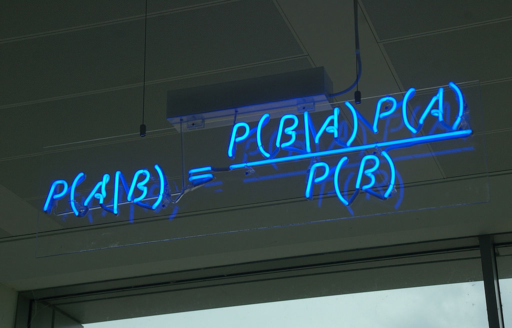
The Naive Bayes classifier returns the class that as the maximum posterior probability given the features:

where \(y\) it’s a class and \(\vec{x}\) is a feature vector associated to an observation.

The NB classifier is based on Bayes’ theorem. Applying the theorem to the equation above, we get:

In training, when iterating over all classes, for a given observation, and calculating the probabilities above, the probability of the observation, i.e., the denominator, is always the same, it has no influence, so we can then simplify the formula:

which, if we decompose the vector of features, is the same as:

this is hard to compute because it involves estimating every possible combination of features. We can relax this computation by applying the Naive Bayes assumption, which states that:

formerly, \(p(x_{i} \mid y,x_{j}) = p(x_{i} \mid y)\) with \(i \neq j\). The probabilities \(p(x_{i} \mid y)\) are independent given the class \(y\) and hence can be ‘naively’ multiplied:

plugging this into our equation:

we get the final Naive Bayes model, which as a consequence of the assumption above, doesn’t capture dependencies between each input variable in \(\vec{x}\).

Trainning

Training in Naive Bayes is mainly done by counting features and classes. Note that the procedure described below needs to be done for every class \(y_{i}\).

To calculate the prior, we simply count how many samples in the training data fall into each class $y_{i}$ divided by the total number of samples:

To calculate the likelihood estimate, we count the number of times a feature \(w_{i}\) appears among all features in all samples of class \(y_{i}\):

This will result in a big table of occurrences of features for all classes in the training data.

Classification

When given a new sample to classify, and assuming that it contains features \(x_{1}, x_{3}, x_{5}\), we need to compute, for each class \(y_{i}\):

This is decomposed into:

Again, this is calculated for each class \(y_{i}\), and we assign to the new observed sample the class that has the highest score.

From Naive Bayes to Hidden Markov Models

The model presented before predicts a class for a set of features associated with an observation. To predict a class sequence \(y=(y_{1}, \dots, y_{n})\) for a sequence of observations \(x=(x_{1}, \dots, y_{n})\), a simple sequence model can be formulated as a product over single Naïve Bayes models:

Two aspects of this model:

• there is only one feature at each sequence position, namely the identity of the respective observation due to the assumption that each feature is generated independently, conditioned on the class \(y_{i}\).

• it doesn’t capture interactions between the observable variables \(x_{i}\).

It is reasonable to assume that there are dependencies at consecutive sequence positions \(y_{i}\), remember the example above about the part-of-speech tags?

This is where the First-order Hidden Markov Model appears, introducing the Markov Assumption:

which is written in its more general form:

where Y represents the set of all possible label sequences \(\vec{y}\).

Hidden Markov Model

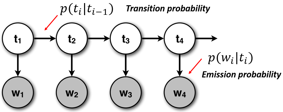
A Hidden Markov Model (HMM) is a sequence classifier. As other machine learning algorithms it can be trained, i.e.: given labeled sequences of observations, and then using the learned parameters to assign a sequence of labels given a sequence of observations. Let’s define an HMM framework containing the following components:

• states (e.g., labels): \(T = t_{1}, t_{2}, \ldots, t_{N}\)
• observations (e.g., words) : \(W = w_{1}, w_{2}, \ldots, w_{N}\)
• two special states: \(t_{start}\) and \(t_{end}\) which are not associated with the observation

and probabilities relating states and observations:

• initial probability: an initial probability distribution over states
• final probability: a final probability distribution over states
• transition probability: a matrix \(A\) with the probabilities from going from one state to another
• emission probability: a matrix \(B\) with the probabilities of an observation being generated from a state

A First-order Hidden Markov Model has the following assumptions:

• Markov Assumption: the probability of a particular state is dependent only on the previous state. Formally: \(P(t_{i} \mid t_{1}, \ldots, t_{i-1}) = P(t_{i} \mid t_{i-1})\)

• Output Independence: the probability of an output observation \(w_{i}\) depends only on the state that produced the observation \(t_{i}\) and not on any other states or any other observations. Formally: \(P(w_{i} \mid t_{1} \ldots q_{i}, \ldots, q_{T} ,o_{1}, \ldots,o_{i}, \ldots,o_{T} ) = P(o_{i} \mid q_{i})\)

Notice how the output assumption is closely related with the Naive Bayes classifier presented before. The figure below makes it easier to understand the dependencies and the relationship with the Naive Bayes classifier:

We can now define two problems which can be solved by an HMM, the first is learning the parameters associated with a given observation sequence, that is training. For instance given words of a sentence and the associated part-of-speech tags, one can learn the latent structure.

The other one is applying a trained HMM to an observation sequence, for instance, having a sentence, predicting each word’s part-of-speech tag, using the latent structure from the training data learned by the HMM.

Learning: estimating transition and emission matrices

Given an observation sequence \(W\) and the associated states \(T\) how can we learn the HMM parameters, that is, the matrices \(A\) and \(B\)?

Using an HHM in a supervised scenario is done by applying the Maximum Likelihood Estimation principle, which will compute the matrices.

This is achieved by counting how many times each event occurs in the corpus and normalising the counts to form proper probability distributions. We need to count 4 quantities which represent the counts of each event in the corpus:

Initial counts: \(\displaystyle C_{\text{init}} (t_{k}) = \sum_{m=1}^{M} 1(t_{1}^m = t_{k})\)
(how often does state \(t_{k}\) is the initial state)

Transition counts: \(\displaystyle C_{\text{trans}} (t_{k}, t_{l}) = \sum_{m=1}^{M} \sum_{m=2}^N 1(t_{i}^{m} = t_{k} ∧ t_{i-1}^{m} = t_{l})\)
(how often does state \(t_{k}\) transits to another state \(t_{l}\))

Final Counts: \(\displaystyle C_{\text{final}} (t_{k}) = \sum_{m=1}^{M} 1(t_{N}^m = t_{k})\)
(how often does state \(t_{k}\) is the final state)

Emissions counts: \(\displaystyle C_{\text{emiss}} (w_{j},t_{k}) = \sum_{m=1}^{M} \sum_{i=1}^N 1(x_{i}^{m} = w_{j} ∧ t_{i}^{m} = t_{k})\)
(how often does state \(t_{k}\) is associated with the observation/word \(w_{j}\))

where, \(M\) is the number of training examples and \(N\) is the length of the sequence, 1 is an indicator function that has the value 1 when the particular event happens, and 0 otherwise. The equations scan the training corpus and count how often each event occurs.

All these 4 counts are then normalised in order to have proper probability distributions:

These equations will produce the transition probability matrix \(A\), with the probabilities from going from one label to another and the emission probability matrix \(B\) with the probabilities of an observation being generated from a state.

Laplace smoothing

How will the model handle words not seen during training?

In the presence of an unseen word/observation, \(P(W_{i} \mid T_{i}) = 0\) and has a consequence incorrect decisions will be made during the predicting process.

There is a technique to handle these situations called Laplace smoothing or additive smoothing. The idea is that every state will always have a small emission probability of producing an unseen word, for instance, denoted by UNK. Every time the HMM encounters an unknown word it will use the value \(P(\text{UNK} \mid T_{i})\) as the emission probability.

Decoding: finding the hidden state sequence for an observation

Given a trained HMM i.e., the transition matrixes \(A\) and \(B\), and a new observation sequence \(W = w_{1}, w_{2}, \ldots, w_{N}\) we want to find the sequence of states \(T = t_{1}, t_{2}, \ldots, t_{N}\) that best explains it.

This is can be achieved by using the Viterbi algorithm, which finds the best state assignment to the sequence \(T_{1} \ldots T_{N}\) as a whole. There is another algorithm, Posterior Decoding which consists in picking the highest state posterior for each position \(i\) in the sequence independently.

Viterbi

It’s a dynamic programming algorithm for computing:

the score of a best path up to position \(i\) ending in state \(t\). The Viterbi algorithm tackles the equation above by using the Markov assumption and defining two functions:

the most likely previous state for each state (store a back-trace):

The Viterbi algorithm uses a representation of the HMM called a trellis, which unfolds all possible states for each position and it makes explicit the independence assumption: each position only depends on the previous position.

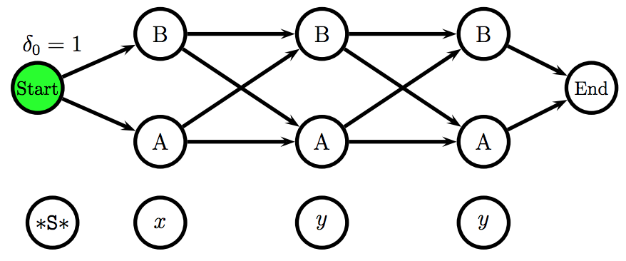
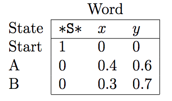
Using the Viterbi algorithm and the emission and transition probabilities matrices, one can fill in the trellis scores and effectively find the Viterbi path.

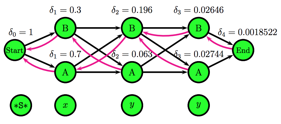
The figures above were taken from a Viterbi algorithm example by Roger Levy for the Linguistics/CSE 256 class. You can find the full example here.

HMM Important Observations

• The main idea of this post was to see the connection between the Naive Bayes classifier and the HMM as a sequence classifier

• If we make the hidden state of HMM fixed, we will have a Naive Bayes model.

• There is only one feature at each word/observation in the sequence, namely the identity i.e., the value of the respective observation.

• Each state depends only on its immediate predecessor, that is, each state \(t_{i}\) is independent of all its ancestors \(t_{1}, t_{2}, \dots, t_{i-2}\) given its previous state \(t_{i-1}\).

• Each observation variable \(w_{i}\) depends only on the current state \(t_{i}\).

Software Packages

• seqlearn: a sequence classification library for Python which includes an implementation of Hidden Markov Models, it follows the sklearn API.

• NLTK HMM: NLTK also contains a module which implements a Hidden Markov Models framework.

• lxmls-toolkit: the Natural Language Processing Toolkit used in the Lisbon Machine Learning Summer School also contains an implementation of Hidden Markov Models.

References

• Machine Learning for Sequential Data: A Review by Thomas G. Dietterich

• Chapter 6: “Naive Bayes and Sentiment Classification” in Speech and Language Processing. Daniel Jurafsky & James H. Martin. Draft of August 7, 2017.

• A Tutorial on Hidden Markov Models and Selected Applications in Speech Recognition

• LxMLS - Lab Guide July 16, 2017 - Day 2 “Sequence Models”

• Chapter 9: “Hidden Markov Models” in Speech and Language Processing. Daniel Jurafsky & James H. Martin. Draft of August 7, 2017.

• Hidden Markov Model inference with the Viterbi algorithm: a mini-example

Extra

There is also a very good lecture, given by Noah Smith at LxMLS2016 about Sequence Models, mainly focusing on Hidden Markov Models and it’s applications from sequence learning to language modelling.

Related posts

• Maximum Entropy Markov Models and Logistic Regression

• Conditional Random Fields for Sequence Prediction

• StanfordNER - training a new model and deploying a web service